Calculation Methods for Logistic Regression

Unlike linear regression, where finding parameters involves solving a system of linear equations, parameter calculation for logistic regression requires the solution of a system of nonlinear equations. The equations become nonlinear because each prediction from the logistic regression model has its own estimated variance; the particular variance estimate influences the prediction, while the estimated prediction influences the estimated variance. The only way to find a solution to these nonlinear equations involves using an iterative, gradient-based algorithm.

For finding the parameters to a logistic regression model, the Business Analysis Module supplies two classes: RWLogisticIterLSQ and RWLogisticLevenbergMarquardt. The following sections provide a brief description of the method encapsulated by each class, along with its pros and cons.

Class RWLogisticIterLSQ uses iterative least squares for finding logistic regression parameters. Some people also refer to this algorithm as the Newton-Raphson method. The algorithm starts with a set of parameters

that corresponds to a linear fit of the data using the normal equations. Then the method repeatedly forms

at iteration k by solving the linear equations:

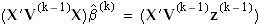
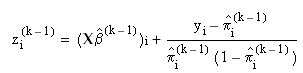
where X is the regression matrix, V(k – 1) is the diagonal matrix of variance estimates at iteration k – 1, and z(k – 1) is a vector of adjusted predictions at iteration k – 1. Element i of z(k – 1) is defined as:


Pros:	Iterative least squares is one of the fastest algorithms for finding logistic regression parameters.
Cons:	If the initial parameter estimate is poor, the algorithm is not guaranteed to converge successfully, while a more sophisticated algorithm might converge.

Class RWLogisticLevenbergMarquardt finds logistic regression parameters using a more sophisticated technique than iterative least squares. It implements what is known as the Levenberg-Marquardt method. The extra sophistication of this algorithm often causes a recovery from poor initial estimates for

. The starting vector of parameters

is the same as for iterative least squares, and at each iteration, the algorithm tries to take a step that is similar to the one taken by iterative least squares. However, it checks to make sure that the step improves the likelihood of the model producing the data. If the step does improve likelihood, the step is taken. If the step does not improve likelihood, the algorithm tries a modified step that falls closer to the gradient. This process of checking and trying a step even closer to the gradient repeats until a step is found that finally improves the likelihood. For further discussion of this and similar optimization algorithms, see Dennis & Schnabel, Numerical Methods for Unconstrained Optimization and Nonlinear Equations, Prentice-Hall, (1983).


Pros:	If the initial parameter estimate is poor, the algorithm often still converges to a set of finite-valued parameters, while iterative least squares may not.
Cons:	The algorithm is slower than iterative least squares.