Decision Trees
Decision trees are data mining methods for predicting a single response variable based on multiple predictor variables. If the response variable is categorical or discrete, the data mining problem is one of classification; whereas if the response is continuous, the problem is a type of regression. Decision trees are generally applicable in both situations. This module includes four of the most widely used algorithms for decision trees:
- C4.5 (imsl.data_mining.C45DecisionTree())
- ALACART (imsl.data_mining.ALACARTDecisionTree())
- CHAID (imsl.data_mining.CHAIDDecisionTree())
- QUEST (imsl.data_mining.QUESTDecisionTree())
The method predict in each class applies a decision tree to a new set of data.
Missing Values
Any observation or case with a missing response variable is eliminated from the analysis. If a predictor has a missing value, each algorithm will skip that case when evaluating the given predictor. When making a prediction for a new case, if the split variable is missing, the prediction function applies surrogate split-variables and splitting rules in turn, if they are estimated with the decision tree. Otherwise, the prediction function returns the prediction from the most recent non-terminal node. In this implementation, only ALACART estimates surrogate split variables when requested.
An Example
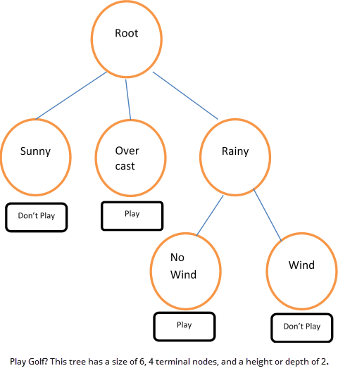
A trivial but illustrative example of the use of a decision tree would be the decision to play golf or not, depending on the weather. The training data, from Quinlan ([1]), is given in the Golf Training Data table below and a decision tree fit to the data is shown in the following figure. Other examples include predicting the chance of survival for heart attack patients based on age, blood pressure and other vital signs; scoring loan applications based on credit history, income, and education; classifying an email as spam based on its characteristics, and so on.
Tree-growing algorithms have similar steps: starting with all observations in a root node, a predictor variable is selected to split the dataset into two or more child nodes or branches. The form of the split depends on the type of predictor and on specifics of the algorithm. If the predictor is categorical, taking discrete values {A, B, C, D} for example, the split may consist of two or more proper subsets, such as {A}, {B, C}, and {D}. If the predictor is continuous, a split will consist of two or more intervals, such as X <= 2, X > 2. The splitting procedure is then repeated for each child node and continued in such manner until one of several possible stopping conditions is met. The result of the decision tree algorithm is a tree structure with a root and a certain number of branches (or nodes). Each branch defines a subset or partition of the data and, conditional on that subset of data, a predicted value for the response variable. A traversal of a branch of the tree thus leads to a prediction, or decision about the response variable. To predict a new out of sample observation, we find the terminal node to which the observation belongs by traversing the tree and finding the data subset (branch) that contains the observation.
For example, the decision tree in the figure can be expressed as a set of rules: If the weather is sunny, don’t play golf. If the weather is overcast, play golf. If the weather is rainy and there is no wind, play golf. On the other hand, if it is rainy and windy, don’t play golf.
Decision trees are intuitive and can be very effective predictive tools. As with any predictive model, a decision tree should be tested on hold-out datasets or refined using K-fold cross-validation to prevent over-fitting.
Golf Training Data
Outlook Temperature Humidity Wind Play sunny 85 85 FALSE don’t play sunny 80 90 TRUE don’t play overcast 83 78 FALSE play rainy 70 96 FALSE play rainy 68 80 FALSE play rainy 65 70 TRUE don’t play overcast 64 65 TRUE play sunny 72 95 FALSE don’t play sunny 69 70 FALSE play rainy 75 80 FALSE play sunny 75 70 TRUE play overcast 72 90 TRUE play overcast 81 75 FALSE play rainy 71 80 TRUE don’t play overcast 81 75 FALSE play rainy 71 80 TRUE don’t play
References
| [1] | Quinlan, J. R. (1993). C4.5 Programs for Machine Learning, Morgan Kaufmann. For the latest information on Quinlan’s algorithms see http://www.rulequest.com/. |