Assembly: ImslCS (in ImslCS.dll) Version: 6.5.0.0
 Syntax
| C# |
|---|
[SerializableAttribute] public class CategoricalGenLinModel |
| Visual Basic (Declaration) |
|---|
<SerializableAttribute> _ Public Class CategoricalGenLinModel |
| Visual C++ |
|---|
[SerializableAttribute] public ref class CategoricalGenLinModel |
Remarks
Reweighted least squares is used to compute (extended) maximum likelihood estimates in some generalized linear models involving categorized data. One of several models, including probit, logistic, Poisson, logarithmic, and negative binomial models, may be fit for input point or interval observations. (In the usual case, only point observations are observed.)
Let
The models available in CategoricalGenLinModel are:
| Model Name | Parameterization | Response PDF |
|---|---|---|
| Model0 (Poisson) |
|
|
| Model1 (Negative Binomial) |
|
|
| Model2 (Logarithmic) |
|
|
| Model3 (Logistic) |
|
|
| Model4 (Probit) |
|
|
| Model5 (Log-log) |
|
|
Here ![]() denotes the cumulative normal
distribution, N and S are known parameters specified for
each observation via column OptionalDistributionParameterColumn of x, and w is an optional fixed parameter specified for each
observation via column FixedParameterColumn of
x. (By default N is taken to be 1 for model
= 0, 3, 4 and 5 and S is taken to be 1 for model = 1.
By default w is taken to be 0.) Since the log-log model (model
= 5) probabilities are not symmetric with respect to 0.5,
quantitatively, as well as qualitatively, different models result when
the definitions of "success" and "failure" are interchanged in this
distribution. In this model and all other models involving
denotes the cumulative normal
distribution, N and S are known parameters specified for
each observation via column OptionalDistributionParameterColumn of x, and w is an optional fixed parameter specified for each
observation via column FixedParameterColumn of
x. (By default N is taken to be 1 for model
= 0, 3, 4 and 5 and S is taken to be 1 for model = 1.
By default w is taken to be 0.) Since the log-log model (model
= 5) probabilities are not symmetric with respect to 0.5,
quantitatively, as well as qualitatively, different models result when
the definitions of "success" and "failure" are interchanged in this
distribution. In this model and all other models involving ![]() ,
, ![]() is taken to be the
probability of a "success."
is taken to be the
probability of a "success."
Note that each row vector in the data matrix can represent a single observation; or, through the use of column FrequencyColumn of the matrix x, each vector can represent several observations.
Computational Details
For interval observations, the probability of the observation is
computed by summing the probability distribution function over the range
of values in the observation interval. For right-interval observations,
![]() is computed as a sum based upon the
equality
is computed as a sum based upon the
equality ![]() . Derivatives
are similarly computed. CategoricalGenLinModel allows three types
of interval observations. In full interval observations, both the lower
and the upper endpoints of the interval must be specified. For
right-interval observations, only the lower endpoint need be given while
for left-interval observations, only the upper endpoint is given.
. Derivatives
are similarly computed. CategoricalGenLinModel allows three types
of interval observations. In full interval observations, both the lower
and the upper endpoints of the interval must be specified. For
right-interval observations, only the lower endpoint need be given while
for left-interval observations, only the upper endpoint is given.
The computations proceed as follows:
- The input parameters are checked for consistency and validity.
- Estimates of the means of the "independent" or design variables are
computed. The frequency of the observation in all but the binomial
distribution model is taken from column FrequencyColumn of the
data matrix x. In binomial distribution models, the
frequency is taken as the product of n =
x[i,OptionalDistributionParameterColumn] and
x[i,FrequencyColumn]. In all cases these values default to 1.
Means are computed as

- If init = 0, initial estimates of the
coefficients are obtained (based upon the observation intervals) as
multiple regression estimates relating transformed observation
probabilities to the observation design vector. For example, in the
binomial distribution models,
 for point
observations may be estimated as
and, when model = 3, the linear relationship is given by
for point
observations may be estimated as
and, when model = 3, the linear relationship is given by![\hat{\theta}=x[i,LowerEndpointColumn]/x[i,
OptionalDistributionParameterColumn]](eqn/eqn_2367.png) while if model = 4,
while if model = 4,

For bounded interval observations, the midpoint of the interval is used for x[i,LowerEndpointColumn]. Right-interval observations are not used in obtaining initial estimates when the distribution has unbounded support (since the midpoint of the interval is not defined). When computing initial estimates, standard modifications are made to prevent illegal operations such as division by zero.
Regression estimates are obtained at this point, as well as later, by use of linear regression.
- Newton-Raphson iteration for the maximum likelihood estimates is
implemented via iteratively reweighted least squares. Let
denote the log of the probability of the i-th observation for coefficients

 . In the least-squares model, the
weight of the i-th observation is taken as the absolute value of
the second derivative of
with respect to(times the frequency of the observation), and the dependent variable is taken as the first derivative
. In the least-squares model, the
weight of the i-th observation is taken as the absolute value of
the second derivative of
with respect to(times the frequency of the observation), and the dependent variable is taken as the first derivative
 with respect to
 , divided by the square root of the weight
times the frequency. The Newton step is given by
where all derivatives are evaluated at the current estimate of
, divided by the square root of the weight
times the frequency. The Newton step is given by
where all derivatives are evaluated at the current estimate of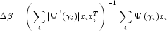
 , and
, and  . This step is computed as the estimated regression
coefficients in the least-squares model. Step halving is used when
necessary to ensure a decrease in the criterion.
. This step is computed as the estimated regression
coefficients in the least-squares model. Step halving is used when
necessary to ensure a decrease in the criterion. - Convergence is assumed when the maximum relative change in any coefficient update from one iteration to the next is less than ConvergenceTolerance or when the relative change in the log-likelihood from one iteration to the next is less than ConvergenceTolerance/100. Convergence is also assumed after MaxIterations or when step halving leads to a step size of less than .0001 with no increase in the log-likelihood.
- For interval observations, the contribution to the log-likelihood is the log of the sum of the probabilities of each possible outcome in the interval. Because the distributions are discrete, the sum may involve many terms. The user should be aware that data with wide intervals can lead to expensive (in terms of computer time) computations.
If InfiniteEstimateMethod is set to 0, then the methods of Clarkson and Jennrich (1991) are used to check for the existence of infinite estimates in
As an example of a situation in which infinite estimates can occur, suppose that observation j is right censored with
 in a logistic model. If design matrix x is such that
  and
and  for all
  , then the
optimal estimate of
, then the
optimal estimate of  occurs at
leading to an infinite estimate of both
occurs at
leading to an infinite estimate of both and
and  . In CategoricalGenLinModel, such
estimates may be "computed."
In all models fit by CategoricalGenLinModel, infinite estimates
can only occur when the optimal estimated probability associated with
the left- or right-censored observation is 1. If
InfiniteEstimateMethod is set to 0, left- or right- censored
observations that have estimated probability greater than 0.995 at some
point during the iterations are excluded from the log-likelihood, and
the iterations proceed with a log-likelihood based upon the remaining
observations. This allows convergence of the algorithm when the maximum
relative change in the estimated coefficients is small and also allows
for the determination of observations with infinite
At convergence, linear programming is used to ensure that the eliminated observations have infinite
. In CategoricalGenLinModel, such
estimates may be "computed."
In all models fit by CategoricalGenLinModel, infinite estimates
can only occur when the optimal estimated probability associated with
the left- or right-censored observation is 1. If
InfiniteEstimateMethod is set to 0, left- or right- censored
observations that have estimated probability greater than 0.995 at some
point during the iterations are excluded from the log-likelihood, and
the iterations proceed with a log-likelihood based upon the remaining
observations. This allows convergence of the algorithm when the maximum
relative change in the estimated coefficients is small and also allows
for the determination of observations with infinite
At convergence, linear programming is used to ensure that the eliminated observations have infinite . If some (or all)
of the removed observations should not have been removed (because their
estimated
. If some (or all)
of the removed observations should not have been removed (because their
estimated  must be finite), then the
iterations are restarted with a log-likelihood based upon the finite
observations. See Clarkson and Jennrich
(1991) for more details.
must be finite), then the
iterations are restarted with a log-likelihood based upon the finite
observations. See Clarkson and Jennrich
(1991) for more details.When InfiniteEstimateMethod is set to 1, no observations are eliminated during the iterations. In this case, when infinite estimates occur, some (or all) of the coefficient estimates
 will become large, and it is likely that the Hessian will
become (numerically) singular prior to convergence.
will become large, and it is likely that the Hessian will
become (numerically) singular prior to convergence.When infinite estimates for the
 are
detected, linear regression (see Chapter 2, Regression;) is used at the
convergence of the algorithm to obtain unique estimates
are
detected, linear regression (see Chapter 2, Regression;) is used at the
convergence of the algorithm to obtain unique estimates  . This is accomplished by regressing the optimal
or the observations with finite
. This is accomplished by regressing the optimal
or the observations with finite
 against
  , yielding
a unique
, yielding
a unique  (by setting coefficients
that are linearly related to previous
coefficients in the model to zero). All of the final statistics relating
to are based upon these estimates.
(by setting coefficients
that are linearly related to previous
coefficients in the model to zero). All of the final statistics relating
to are based upon these estimates.
Residuals are computed according to methods discussed by Pregibon (1981). Let
 denote the
log-likelihood of the i-th observation evaluated at
. Then, the standardized residual is
computed as
where
denote the
log-likelihood of the i-th observation evaluated at
. Then, the standardized residual is
computed as
where
 is the value of
  when evaluated at the optimal and the derivatives here (and only here) are with respect to
rather than with respect to
when evaluated at the optimal and the derivatives here (and only here) are with respect to
rather than with respect to  . The denominator of this expression is used as the "standard
error of the residual" while the numerator is the "raw" residual.
. The denominator of this expression is used as the "standard
error of the residual" while the numerator is the "raw" residual.Following Cook and Weisberg (1982), we take the influence of the i-th observation to be
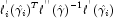
This quantity is a one-step approximation to the change in the estimates when the i-th observation is deleted. Here, the partial derivatives are with respect to
.
Programming Notes
- Classification variables are specified via ClassificationVariableColumn. Indicator or dummy variables are created for the classification variables.
- To enhance precision "centering" of covariates is performed if ModelIntercept is set to 1 and (number of observations) - (number of rows in x missing one or more values) > 1. In doing so, the sample means of the design variables are subtracted from each observation prior to its inclusion in the model. On convergence the intercept, its variance and its covariance with the remaining estimates are transformed to the uncentered estimate values.
- Two methods for specifying a binomial distribution model are possible. In the first method, x[i,FrequencyColumn] contains the frequency of the observation while x[i,LowerEndpointColumn] is 0 or 1 depending upon whether the observation is a success or failure. In this case, N = x[i,OptionalDistributionParameterColumn] is always 1. The model is treated as repeated Bernoulli trials, and interval observations are not possible.
A second method for specifying binomial models is to use x[i,LowerEndpointColumn] to represent the number of successes in the x[i,OptionalDistributionParameterColumn] trials. In this case, x[i,FrequencyColumn] will usually be 1, but it may be greater than 1, in which case interval observations are possible.
Note that the Solve()()() method must be called before using any property as a right operand, otherwise the value is null.