PROP_HAZARDS_GEN_LIN Function (PV-WAVE Advantage)
Analyzes survival and reliability data using Cox’s proportional hazards model.
Usage
result = PROP_HAZARDS_GEN_LIN (x, n_var_effects, indices_effects, max_class)
Input Parameters
x—Array of length n_observations by n_columns containing the data, where n_observations is the number of observations and n_columns is the number of columns in x. When keyword Ties_option = 1, the observations in x must be grouped by stratum and sorted from largest to smallest failure time within each stratum, with the strata separated.
n_var_effects—Array of length Nef containing the number of variables associated with each effect in the model, where Nef is the number of effects in the model.
indices_effects—Index array of length n_var_effects(0) + ... + n_var_effects(Nef–1) containing the column indices of x associated with each effect. The first n_var_effects(0) elements of indices_effects contain the column indices of x for the variables in the first effect. The next n_var_effects(1) elements in indices_effects contain the column indices for the second effect, etc.
max_class—An upper bound on the total number of different values found among the classification variables in x. For example, if the model consisted of two class variables, one with the values {1, 2, 3, 4} and a second with the values {0, 1}, then then the total number of different classification values is 4+2=6, and max_class ≥ 6.
Returned Value
result—Array of length ncoef by 4 containing the parameter estimates and associated statistics.

1—Coefficient estimate

.
2—Estimated standard deviation of the estimated coefficient.
3—Asymptotic normal score for testing that the coefficient is zero against the two-sided alternative.
4—
p-value associated with the normal score in column 3.
ncoef is the number of estimated coefficients in the model.
Input Keywords
Double—If present and nonzero, double precision is used.
Maxit—Maximum number of iterations. Maxit = 30 will usually be sufficient. Use Maxit = 0 to compute the Hessian and gradient, stored in Variance_covariance_matrix and Update, at the initial estimates. When Maxit = 0, initial_est_input must be used. Default: Max_iterations = 30.
Convergence_eps—Convergence criterion. Convergence is assumed when the relative change in Maximum_likelihood from one iteration to the next is less than Convergence_eps. If Convergence_eps is zero, Convergence_eps = 0.0001 is assumed. Default: Convergence_eps = 0.0001.
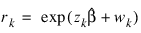
Ratio—Ratio at which a stratum is split into two strata. Default: Ratio = 1000.0. Let:
be the observation proportionality constant, where zk is the design row vector for the kth observation and wk is the optional fixed parameter specified by xk, Constant_col. Let rmin be the minimum value rk in a stratum, where, for failed observations, the minimum is over all times less than or equal to the time of occurrence of the kth observation. Let rmax be the maximum value of rk for the remaining observations in the group. Then, if rmin > Ratio rmin, the observations in the group are divided into two groups at k. Ratio = 1000 is usually a good value. Set Ratio = –1.0 if no division into strata is to be made.
X_response_col—Column index in x containing the response variable. For point observations, xi, X_response_col contains the time of the ith event. For right-censored observations, xi, X_response_col contains the right-censoring time. Note that because PROP_HAZARDS_GEN_LIN only uses the order of the events, negative “times” are allowed. Default: X_response_col = 0.
Censor_codes_col—Column index in x containing the censoring code for each observation. Default: A censoring code of 0 is assumed for all observations.
0—Exact censoring time
xi, X_response_col.
1—Right censored. The exact censoring time is greater than
xi,X_response_col.
Stratification_col—Column index in x containing the stratification variable. Column Stratification_col in x contains a unique number for each stratum. The risk set for an observation is determined by its stratum. Default: All observations are considered to be in one stratum.
Constant_col—Column index in
x containing a constant,
wi, to be added to the linear response. The linear response is taken to be

where
wi is the observation constant,
zi is the observation design row vector, and

is the vector of estimated parameters. The “fixed” constant allows you to test hypotheses about parameters via the log-likelihoods. Default:
wi is assumed to be 0 for all observations.
Freq_response_col—Column index in x containing the number of responses for each observation. Default: A response frequency of 1 for each observation is assumed.
Ties_option—Method for handling ties. Default: Ties_option = 0.
0
—Breslow’s approximate method.
1
—Failures are assumed to occur in the same order as the observations input in
x. The observations in
x must be sorted from largest to smallest failure time within each stratum, and grouped by stratum. All observations are treated as if their failure/censoring times were distinct when computing the log-likelihood.
Initial_est_input—An array of length ncoef containing the initial estimates on input to PROP_HAZARDS_GEN_LIN, where ncoef is the number of estimated coefficients in the model. Default: all initial estimates are taken to be 0.
Index_class_var—An index array of length n_class_var containing the column numbers of x that are the classification variables.
Output Keywords
Maximum_likelihood—The maximized log-likelihood.
N_missing—Number of rows of data in x that contain missing values in one or more columns X_response_col, Freq_response_col, Constant_col, Censor_codes_col, Stratification_col, Index_class_var, or indices_effects of x.
Case_statistics—Array of length n_observations by 5 containing the case statistics for each observation.
1—Estimated survival probability at the observation time.
2—Estimated observation influence or leverage.
3—A residual estimate.
4—Estimated cumulative baseline hazard rate.
5—Observation proportionality constant.
X_mean—Array of length ncoef containing the means of the design variables, where ncoef is the number of estimated coefficients in the model.
Variance_covariance_matrix—Array of length ncoef by ncoef containing the estimated asymptotic variance-covariance matrix of the parameters, where ncoef is the number of estimated coefficients in the model. For Maxit = 0, the return value is the inverse of the Hessian of the negative of the log-likelihood, computed at the estimates input in Initial_est_input.
Updates—Array of length ncoef containing the last parameter updates (excluding step halvings), where ncoef is the number of estimated coefficients in the model. For Maxit = 0, Updates contains the inverse of the Hessian times the gradient vector computed at the estimates input in Initial_est_input.
Stratum_number—Array of length n_observations giving the stratum number used for each observation. If Ratio is not –1.0, additional “strata” (other than those specified by column Stratification_col of x) may be generated. Stratum_number also contains a record of the generated strata.
N_class_values—Array of length n_class_var containing the number of values taken by each classification variable, where n_class_var is the number of elements in Index_class_var. N_class_values(i) is the number of distinct values for the ith classification variable. Must be used with Index_class_var.
Class_values—Array of length N_class_values(0) + N_class_values(1) + ... + N_class_values(N_class_var–1) containing the distinct values of the classification variables. The first N_class_values(0) elements of Class_values contain the values for the first classification variable, the next N_class_values(1) elements contain the values for the second classification variable, and so forth. Must be used with Index_class_var and N_class_values.
Discussion
PROP_HAZARDS_GEN_LIN computes parameter estimates and other statistics in Proportional Hazards Generalized Linear Models. These models were first proposed by Cox (1972). Two methods for handling ties are allowed in PROP_HAZARDS_GEN_LIN. Time-dependent covariates are not allowed. The user is referred to Cox and Oakes (1984), Kalbfleisch and Prentice (1980), Elandt-Johnson and Johnson (1980), Lee (1980), or Lawless (1982), among other texts, for a thorough discussion of the Cox proportional hazards model.
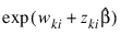
Let λ(t, zi) represent the hazard rate at time t for observation number i with covariables contained as elements of row vector zi. The basic assumption in the proportional hazards model (the proportionality assumption) is that the hazard rate can be written as a product of a time varying function λ0(t), which depends only on time, and a function f(zi), which depends only on the covariable values. The function f(zi) used in PROP_HAZARDS_GEN_LIN is given as f(zi) = exp(wi + βzi) where wi is a fixed constant assigned to the observation, and β is a vector of coefficients to be estimated. With this function one obtains a hazard rate λ(t, zi) = λ0(t) exp(wi + βzi). The form of λ0(t) is not important in proportional hazards models.
The constants wi may be known theoretically. For example, the hazard rate may be proportional to a known length or area, and the wi can then be determined from this known length or area. Alternatively, the wi may be used to fix a subset of the coefficients β (say, β1) at specified values. When wi is used in this way, constants wi = β1z1i are used, while the remaining coefficients in β are free to vary in the optimization algorithm. If user-specified constants are not desired, the user should set Constant_col to 0 so that wi = 0 will be used.
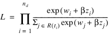
With this definition of λ(t, zi), the usual partial (or marginal, see Kalbfleisch and Prentice (1980)) likelihood becomes:
where R(ti) denotes the set of indices of observations that have not yet failed at time ti (the risk set), ti denotes the time of failure for the ith observation, nd is the total number of observations that fail. Right-censored observations (i.e., observations that are known to have survived to time ti, but for which no time of failure is known) are incorporated into the likelihood through the risk set R(ti). Such observations never appear in the numerator of the likelihood. When Ties_option = 0, all observations that are censored at time ti are not included in R(ti), while all observations that fail at time ti are included in R(ti).
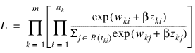
If it can be assumed that the dependence of the hazard rate upon the covariate values remains the same from stratum to stratum, while the time-dependent term, λ0(t), may be different in different strata, then PROP_HAZARDS_GEN_LIN allows the incorporation of strata into the likelihood as follows. Let k index the m = stratification_col strata. Then, the likelihood is given by:
In PROP_HAZARDS_GEN_LIN, the log of the likelihood is maximized with respect to the coefficients β. A quasi-Newton algorithm approximating the Hessian via the matrix of sums of squares and cross products of the first partial derivatives is used in the initial iterations (the “Q-N” method in the output). When the change in the log-likelihood from one iteration to the next is less than 100*convergence_eps, the Newton-Raphson iteration is used (the “N-R” method). If, during any iteration, the initial step does not lead to an increase in the log-likelihood, then step halving is employed to find a step that will increase the log-likelihood.
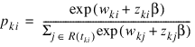
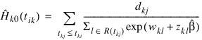
Once the maximum likelihood estimates have been computed, PROP_HAZARDS_GEN_LIN computes estimates of a probability associated with each failure. Within stratum k, an estimate of the probability that the ith observation fails at time ti given the risk set R(tki) is given by:
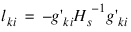
A diagnostic “influence” or “leverage” statistic is computed for each noncensored observation as:
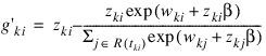
where Hs is the matrix of second partial derivatives of the log-likelihood, and:
is computed as:
Influence statistics are not computed for censored observations.
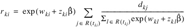
A “residual” is computed for each of the input observations according to methods given in Cox and Oakes (1984, page 108). Residuals are computed as:
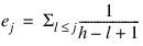
where dkj is the number of tied failures in group k at time tkj. Assuming that the proportional hazards assumption holds, the residuals should approximate a random sample (with censoring) from the unit exponential distribution. By subtracting the expected values, centered residuals can be obtained. (The jth expected order statistic from the unit exponential with censoring is given as:
where h is the sample size, and censored observations are not included in the summation.)
An estimate of the cumulative baseline hazard within group k is given as:
The observation proportionality constant is computed as:
Programming Notes
1. The covariate vectors zki are computed from each row of the input matrix x via REGRESSORS (see Chapter 2, Regression). Thus, class variables are easily incorporated into the zki. The reader is referred to the document for REGRESSORS in the regression chapter for a more detailed discussion. Note that PROP_HAZARDS_GEN_LIN calls REGRESSORS with Dummy_method = 1.
2. The average of each of the explanatory variables is subtracted from the variable prior to computing the product zkiβ. Subtraction of the mean values has no effect on the computed log-likelihood or the estimates since the constant term occurs in both the numerator and denominator of the likelihood. Subtracting the mean values does help to avoid invalid exponentiation in the algorithm and may also speed convergence.
3. PROP_HAZARDS_GEN_LIN allows for two methods of handling ties. In the first method (Ties_option = 1), the user is allowed to break ties in any manner desired. When this method is used, it is assumed that the user has sorted the rows in x from largest to smallest with respect to the failure/censoring times xi, X_response_col within each stratum (and across strata), with tied observations (failures or censored) broken in the manner desired. The same effect can be obtained with Ties_option = 0 by adding (or subtracting) a small amount from each of the tied observations failure/ censoring times ti = xi, X_response_col so as to break the ties in the desired manner.
The second method for handling ties (Ties_option = 0) uses an approximation for the tied likelihood proposed by Breslow (1974). The likelihood in Breslow’s method is as specified above, with the risk set at time ti including all observations that fail at time ti, while all observations that are censored at time ti are not included. (Tied censored observations are assumed to be censored immediately prior to the time ti).
4. If Initial_est_input option is used, then it is assumed that the user has provided initial estimates for the model coefficients β in Initial_est_input. When initial estimates are provided by the user, care should be taken to ensure that the estimates correspond to the generated covariate vector zki. If Initial_est_input option is not used, then initial estimates of zero are used for all of the coefficients. This corresponds to no effect from any of the covariate values.
5. If a linear combination of covariates is monotonically increasing or decreasing with increasing failure times, then one or more of the estimated coefficients is infinite and extended maximum likelihood estimates must be computed. Such estimates may be written as

where
ρ =
∞ at the supremum of the likelihood so that

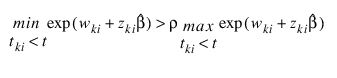
is the finite part of the solution. In PROP_HAZARDS_GEN_LIN, it is assumed that extended maximum likelihood estimates must be computed if, within any group
k, for any time
t:
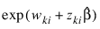
where ρ = Ratio is specified by the user. Thus, for example, if ρ = 10000, then PROP_HAZARDS_GEN_LIN does not compute extended maximum likelihood estimates until the estimated proportionality constant:
is 10000 times larger for all observations prior to t than for all observations after
t. When this occurs, PROP_HAZARDS_GEN_LIN computes estimates for

by splitting the failures in stratum
k into two strata at
t (see Bryson and Johnson 1981). Censored observations in stratum k are placed into a stratum based upon the associated value for:
The results of the splitting are returned in
Stratum_number. The estimates

based upon the stratified likelihood represent the finite part of the extended maximum likelihood solution. PROP_HAZARDS_GEN_LIN does not compute

explicitly, but an estimate for

may be obtained in some circumstances by setting
Ratio = –1 and optimizing the log-likelihood without forming additional strata. The solution

obtained will be such that

for some finite value of
ρ > 0. At this solution, the Newton-Raphson algorithm will not have “converged” because the Newton-Raphson step sizes returned in
Update will be large, at least for some variables. Convergence will be declared, however, because the relative change in the log-likelihood during the final iterations will be small.
Example
The following data is taken from Lawless (1982, page 287) and involve the survival of lung cancer patients based upon their initial tumor types and treatment type. In the first example, the likelihood is maximized with no strata present in the data. This corresponds to Example 7.2.3 in Lawless (1982, page 367). The input data is printed in the output. The model is given as:
where αi and γj correspond to dummy variables generated from column indices 5 and 6 of x, respectively, x1 corresponds to column index 2, x2 corresponds to column index 3, and x3 corresponds to column index 4 of x.
; Number of observations.
nobs= 40
; An upper bound on the total number of different values
; found among the classification variables in x.
maxcl = 10
; Index array containing the column indices of x associated with
; each effect.
indef = [2, 3, 4, 5, 6]
; Array containing the number of variables associated with each
; effect in the model.
nvef = [1, 1, 1, 1, 1]
; An index array containing the column numbers of x
; that are the classification variables.
indcl = [5, 6]
; Ratio at which a stratum is split into two strata.
ratio = 10000.0
; Number of columns in x
ncol = 7
; Number of estimated coefficients in the model.
ncoef = 7
; Initial estimate
incoef = [0.0,0.0,0.0,0.0,0.0,0.0,0.0]
; A 2-D Array containing the data.
y = [ $
411, 0, 7, 64, 5, 1, 0, $
126, 0, 6, 63, 9, 1, 0, $
118, 0, 7, 65, 11, 1, 0, $
92, 0, 4, 69, 10, 1, 0, $
8, 0, 4, 63, 58, 1, 0, $
25, 1, 7, 48, 9, 1, 0, $
11, 0, 7, 48, 11, 1, 0, $
54, 0, 8, 63, 4, 2, 0, $
153, 0, 6, 63, 14, 2, 0, $
16, 0, 3, 53, 4, 2, 0, $
56, 0, 8, 43, 12, 2, 0, $
21, 0, 4, 55, 2, 2, 0, $
287, 0, 6, 66, 25, 2, 0, $
10, 0, 4, 67, 23, 2, 0, $
8, 0, 2, 61, 19, 3, 0, $
12, 0, 5, 63, 4, 3, 0, $
177, 0, 5, 66, 16, 4, 0, $
12, 0, 4, 68, 12, 4, 0, $
200, 0, 8, 41, 12, 4, 0, $
250, 0, 7, 53, 8, 4, 0, $
100, 0, 6, 37, 13, 4, 0, $
999, 0, 9, 54, 12, 1, 1, $
231, 1, 5, 52, 8, 1, 1, $
991, 0, 7, 50, 7, 1, 1, $
1, 0, 2, 65, 21, 1, 1, $
201, 0, 8, 52, 28, 1, 1, $
44, 0, 6, 70, 13, 1, 1, $
15, 0, 5, 40, 13, 1, 1, $
103, 1, 7, 36, 22, 2, 1, $
2, 0, 4, 44, 36, 2, 1, $
20, 0, 3, 54, 9, 2, 1, $
51, 0, 3, 59, 87, 2, 1, $
18, 0, 4, 69, 5, 3, 1, $
90, 0, 6, 50, 22, 3, 1, $
84, 0, 8, 62, 4, 3, 1, $
164, 0, 7, 68, 15, 4, 1, $
19, 0, 3, 39, 4, 4, 1, $
43, 0, 6, 49, 11, 4, 1, $
340, 0, 8, 64, 10, 4, 1, $
231, 0, 7, 67, 18, 4, 1 $
]
; Reform data to match the input requirement
y = TRANSPOSE(REFORM(y, ncol,nobs))
; Call the routine
coef = PROP_HAZARDS_GEN_LIN(y, nvef, indef, maxcl, $
Index_class_var=indcl, $
Censor_codes_col=1, $
Variance_cov=cov, $
Updates=updates, $
Stratum_number=stratum_number, $
Case_statistics=statistics, $
N_class_values=n_class_values, $
Class_values=class_values, $
ratio=1000.0, $
Maximum_likelihood=likehood, $
N_missing=missing, $
X_mean = mean)
; Format the outputs
PRINT, " OUTPUT"
PRINT, ""
PRINT, "Initial Estimates"
PRINT, incoef, Format = '(7F7.5)'
PRINT, ""
PRINT, "LOG-likelihood ", likehood
PRINT, ""
PRINT, " Coefficient Statistics"
PRINT, " Coefficient Standard Asymptotic Asymptotic"
PRINT, " error z-statistic p-value"
FOR i=0L, ncoef - 1 DO $
PRINT, coef(i, 0), coef(i, 1),coef(i, 2), coef(i, 3)
str1 = STRARR(7)
str2 = STRARR(7)
spc = ' '
FOR i=0L, ncoef-1 DO BEGIN & $
FOR j=0L, 4 DO $
IF (j LT i) THEN str1(i) = str1(i) + spc $
ELSE str1(i) = str1(i) + string(cov(i,j)) & $
FOR j=5L, 6 DO $
IF (j LT i) THEN str2(i) = str2(i) + spc $
ELSE str2(i) = str2(i) + string(cov(i,j)) & $
ENDFOR
; Print Coefficient Covariance
PRINT, ""
PRINT, " Asymptotic Coefficient Covariance"
FOR i=0L, 4 DO $
PRINT, str1(i)
PM, str2
PRINT, ""
PRINT, " Case Analysis"
PRINT, " Survial Influence Residual Cumulative Prop."
PRINT, " Probability hazard constant"
PRINT, TRANSPOSE(statistics), Format = '(5F13.2)'
PRINT, ""
PRINT, " Last Coefficient Update"
PRINT, updates(0), updates(1), updates(2),updates(3),updates(4)
PRINT, updates(5), updates(6)
PRINT, ""
PRINT, " Covariate Means"
PRINT, mean(0), mean(1),mean(2),mean(3),mean(4)
PRINT, mean(5), mean(6)
PRINT, ""
n_class = N_ELEMENTS(indcl)
PRINT, " Distinct Values For Each Class Variable"
n1 = n_class_values(0)
n2 = n_class_values(1)
var1 = class_values(0:n1-1)
var2 = class_values(n1:n1+n2-1)
PRINT, "Variable 1: ", FIX(var1)
PRINT, "Variable 2: ", FIX(var2)
PRINT, ""
PRINT, " Stratum Numbers For Each Observation"
PRINT, stratum_number, Format = '(10I5)'
PRINT, ""
PRINT, "Number of Missing Values: ", missing
Output
Initial Estimates
0.000000.000000.000000.000000.000000.000000.00000
LOG-likelihood -87.8878
Coefficient Statistics
Coefficient Standard Asymptotic Asymptotic
error z-statistic p-value
-0.584594 0.136840 -4.27209 1.93119e-05
-0.0130519 0.0205803 -0.634197 0.525952
0.000761767 0.0118179 0.0644585 0.948605
-0.367045 0.484770 -0.757152 0.448959
-0.00772070 0.506751 -0.0152357 0.987844
1.11294 0.633059 1.75804 0.0787414
0.379709 0.405802 0.935701 0.349427
Asymptotic Coefficient Covariance
0.0187252 0.000253001 0.000334516 0.00574491 0.00974995
0.000423548 -4.11981e-05 -0.00166347 -0.000795351
0.000139664 0.000811059 -0.00183122
0.235002 0.0979898
0.256797
0.00426420 0.00208159
-0.00307913 -0.00289804
0.000599460 0.00168395
0.118379 0.0373461
0.125260 -0.0194430
0.400763 0.0628911
0.164675
Case Analysis
Survial Influence Residual Cumulative Prop.
Probability hazard constant
0.00 0.04 2.05 6.10 0.34
0.30 0.11 0.74 1.21 0.61
0.34 0.12 0.36 1.07 0.33
0.43 0.16 1.53 0.84 1.83
0.96 0.56 0.09 0.05 2.05
0.74 NaN 0.13 0.31 0.42
0.92 0.37 0.03 0.08 0.42
0.59 0.26 0.14 0.53 0.27
0.26 0.12 1.20 1.36 0.88
0.85 0.15 0.97 0.17 5.76
0.55 0.31 0.21 0.60 0.36
0.74 0.21 0.96 0.31 3.12
0.03 0.06 3.02 3.53 0.86
0.94 0.09 0.17 0.06 2.71
0.96 0.16 1.31 0.05 28.89
0.89 0.23 0.59 0.12 4.82
0.18 0.09 2.62 1.71 1.54
0.89 0.19 0.33 0.12 2.68
0.14 0.23 0.72 1.96 0.37
0.05 0.09 1.66 2.95 0.56
0.39 0.22 1.17 0.94 1.25
0.00 0.00 1.73 21.10 0.08
0.08 NaN 2.19 2.52 0.87
0.00 0.00 2.46 8.89 0.28
0.99 0.31 0.05 0.01 4.28
0.11 0.17 0.34 2.23 0.15
0.66 0.25 0.16 0.41 0.38
0.87 0.22 0.15 0.14 1.02
0.39 NaN 0.45 0.94 0.48
0.98 0.25 0.06 0.02 2.53
0.77 0.26 1.03 0.26 3.90
0.63 0.35 1.80 0.46 3.88
0.82 0.26 1.06 0.19 5.47
0.47 0.26 1.65 0.75 2.21
0.51 0.32 0.39 0.67 0.58
0.22 0.18 0.49 1.53 0.32
0.80 0.26 1.08 0.23 4.77
0.70 0.16 0.26 0.36 0.73
0.01 0.23 0.87 4.66 0.19
0.08 0.20 0.81 2.52 0.32
Last Coefficient Update
4.64256e-08 8.40790e-09 -7.39568e-09 -2.65050e-07 -1.04526e-07
5.96707e-08 -3.25471e-09
Covariate Means
5.65000 56.5750 15.6500 0.350000 0.275000
0.125000 5.25000
Distinct Values For Each Class Variable
Variable 1: 1 2 3 4
Variable 2: 0 1
Stratum Numbers For Each Observation
1 1 1 1 1 1 1 1 1 1
1 1 1 1 1 1 1 1 1 1
1 1 1 1 1 1 1 1 1 1
1 1 1 1 1 1 1 1 1 1
Number of Missing Values: 0
Version 2017.0
Copyright © 2017, Rogue Wave Software, Inc. All Rights Reserved.