NORMALCDF Function (PV-WAVE Advantage)
Evaluates the standard normal (Gaussian) distribution function. Using a keyword, the inverse of the standard normal (Gaussian) distribution can be evaluated.
Usage
result = NORMALCDF(x)
Input Parameters
x—Expression to evaluate the normal distribution function for.
Returned Value
result—The probability that a normal random variable takes a value less than or equal to x.
Input Keywords
Double—If present and nonzero, double precision is used.
Inverse—If present and nonzero, evaluates the inverse of the standard normal (Gaussian) distribution function. If Inverse is specified, then argument x represents the probability for which the inverse of the normal distribution function is to be evaluated. In this case, x must be in the open interval (0.0, 1.0).
Discussion
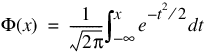
Function NORMALCDF evaluates the distribution function, Φ, of a standard normal (Gaussian) random variable; that is:
The value of the distribution function at the point x is the probability that the random variable takes a value less than or equal to x.
The standard normal distribution (for which NORMALCDF is the distribution function) has mean of zero and variance of 1. The probability that a normal random variable with mean μ and variance σ2 is less than y is given by NORMALCDF evaluated at (y – μ) / σ.
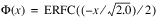
The function
Φ(
x) is evaluated by use of the complementary error function, ERFC (
481). The relationship follows below:
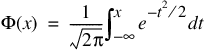
If the keyword Inverse is specified, the NORMALCDF function evaluates the inverse of the distribution function, Φ, of a standard normal (Gaussian) random variable; that is:
NORMALCDF (x, /Inverse ) = Φ–1 (x)
where:
The value of the distribution function at the point x is the probability that the random variable takes a value less than or equal to x. The standard normal distribution has a mean of zero and a variance of 1.
The NORMALCDF function is evaluated by use of minimax rational-function approximations for the inverse of the error function. General descriptions of these approximations are given in Hart et al. (1968) and Strecok (1968). The rational functions used in NORMALCDF are described by Kinnucan and Kuki (1968).
Example
Suppose X is a normal random variable with mean 100 and variance 225. This example finds the probability that X is less than 90 and the probability that X is between 105 and 110.
x1 = (90-100)/15.
p = NORMALCDF(x1)
PM, p, Title = 'The probability that X is less than 90 is:'
; PV-WAVE prints the following:
; The probability that X is less than 90 is: 0.252493
x1 = (105 - 100)/15.
x2 = (110 - 100)/15.
p = NORMALCDF(x2) - NORMALCDF(x1)
PM, p, Title = 'The probability that X is between 105 and 110 is:'
; PV-WAVE prints the following:
; The probability that X is between 105 and 110 is: 0.116949
Version 2017.0
Copyright © 2017, Rogue Wave Software, Inc. All Rights Reserved.