LINLSQ Function (PV-WAVE Advantage)
Solves a linear least-squares problem with linear constraints.
Usage
result = LINLSQ( b, a, c, bl, bu, contype)
Input Parameters
a—Two-dimensional array of size nra by nca containing the coefficients of the least-squares equations, where nra is the number of least-squares equations and nca is the number of variables.
b—One-dimensional array of length nra containing the right-hand sides of the least-squares equations.
c—Two-dimensional array of size ncon by nca containing the coefficients of the constraints, where ncon is the number of constraints.
bl—One-dimensional array of length ncon containing the lower limit of the general constraints. If there is no lower limit on the ith constraint, then bl(i) will not be referenced.
bu—One-dimensional array of length ncon containing the upper limit of the general constraints. If there is no upper limit on the ith constraint, then bu(i) will not be referenced.
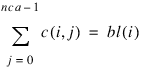
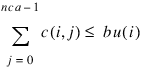
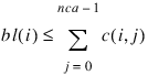
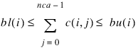
contype—One-dimensional array of length ncon indicating the type of constraints exclusive of simple bounds, where contype(i) = 0, 1, 2, 3 indicates =, ≤ , ≥ , and range constraints, respectively.
Returned Value
result—1D array of length nca containing the approximate solution.
Input Keywords
Double—If present and nonzero, double precision is used.
Xlb—One-dimensional array of length nca containing the lower bound on the variables. If there is no lower bound on the ith variable, then Xlb(i) should be set to 1.0e30.
Xub—One-dimensional array of length nca containing the upper bound on the variables. If there is no upper bound on the ith variable, then Xub(i) should be set to –1.0e30.
Itmax—Set the maximum number of iterations. Default: Itmax = 5*max(nra, nca)
Rel_Tolerance—Relative rank determination tolerance to be used. Default: Rel_Tolerance = SQRT(machine epsilon).
Abs_Tolerance—Absolute rank determination tolerance to be used. Default: Abs_Tolerance = SQRT(machine epsilon).
Output Keywords
Residual—Named variable into which an one-dimensional array containing the residuals b − Ax of the least-squares equations at the approximate solution is stored.
Discussion
The function LINLSQ solves linear least-squares problems with linear constraints. These are systems of least-squares equations of the form:
subject to:
bl ≤ Cx ≤ bu
xl ≤ x ≤ xu
Here A is the coefficient matrix of the least-squares equations, b is the right-hand side, and C is the coefficient matrix of the constraints. The vectors bl, bu, xl and xu are the lower and upper bounds on the constraints and the variables, respectively. The system is solved by defining dependent variables y ≡ Cx and then solving the least-squares system with the lower and upper bounds on x and y. The equation Cx − y = 0 is a set of equality constraints. These constraints are realized by heavy weighting, i.e., a penalty method, Hanson (1986, pp. 826-834).
Example 1
In this example, the following problem is solved in the least-squares sense:
3x1 + 2x2 + x3 = 3.3
4x1 +2x2 + x3 = 2.2
2x1 + 2x2 + x3 = 1.3
x1 + x2 + x3 = 1.0
Subject to:
x1 + x2 + x3 ≤ 1
0 ≤ x1 ≤ 0.5
0 ≤ x2 ≤ 0.5
0 ≤ x3 ≤ 0.5
a = TRANSPOSE([[3.0, 2.0, 1.0], [4.0, 2.0, 1.0], $
[2.0, 2.0, 1.0], [1.0, 1.0, 1.0]])
b = [3.3, 2.3, 1.3, 1.0]
c = [[1.0], [1.0], [1.0]]
xub = [0.5, 0.5, 0.5]
xlb = [0.0, 0.0, 0.0]
contype = [1]
bc = [1.0]
; Note that only upper bound is set for contype =1.
sol = LINLSQ(b, a, c, bc, bc, contype, Xlb = xlb, Xub = xub)
PM, sol, Title = 'Solution'
; PV-WAVE prints the following:
; 0.500000
; 0.300000
; 0.200000
Example 2
The same problem solved in the first example is solved again. This time residuals of the least-squares equations at the approximate solution are returned, and the norm of the residual vector is printed.
a = TRANSPOSE([[3.0, 2.0, 1.0], [4.0, 2.0, 1.0], $
[2.0, 2.0, 1.0], [1.0, 1.0, 1.0]])
b = [3.3, 2.3, 1.3, 1.0]
c = [[1.0], [1.0], [1.0]]
xub = [0.5, 0.5, 0.5]
xlb = [0.0, 0.0, 0.0]
contype = [1]
bc = [1.0]
sol = LINLSQ(b, a, c, bc, bc, contype, Xlb = xlb, $
Xub = xub, Residual = residual)
PM, sol, Title = 'Solution'
; PV-WAVE prints the following:
; Solution
; 0.500000
; 0.300000
; 0.200000
PM, residual, Title = 'Residual'
; PV-WAVE prints the following:
; Residual
; -1.00000
; 0.500000
; 0.500000
; 0.00000
PRINT, 'Norm of Residual =', NORM(residual)
; PV-WAVE prints: Norm of Residual = 1.22474
Version 2017.0
Copyright © 2017, Rogue Wave Software, Inc. All Rights Reserved.