SP_LUFAC Function (PV-WAVE Advantage)
Computes an LU factorization of a sparse matrix stored in either coordinate format or CSC format. Using keywords, any of several related computations can be performed.
Usage
result = SP_LUFAC(a, n_rows)
Input Parameters
a—Sparse matrix stored as an array of structures containing the coefficient matrix A(i,j). See the chapter introduction for a description of structures used for sparse matrices.
n_rows—The number of rows in a.
Returned Value
result—Structure containing the LU factorization of A.
Input Keywords
Transpose—If present and nonzero, ATx = b is solved.
Pivoting—Scalar value specifying the pivoting method to use. For Row Markowitz, set Pivoting to 1; for Column Markowitz, set Pivoting to 2; and for Symmetric Markowitz, set Pivoting to 3. Default: Pivoting = 3
N_search_rows—The number of rows which have the least number of non-zero elements that will be searched for a pivot element. Default: N_search_rows = 3
Iter_refine—If present and nonzero, iterative refinement will be applied.
Tol_drop—Possible fill-in is checked against this tolerance. If the absolute value of the new element is less than Tol_drop, it will be discarded. Default: Tol_drop = 0.0
Stability—The absolute value of the pivot element must be bigger than the largest element in absolute value in its row divided by Stability. Default: Stability = 10.0
Gwth_lim—The computation stops if the growth factor exceeds Gwth_limit. Default: Gwth_limit = 1.0e16
Memory_block—Supply the number of non-zeros which will be added to the factor if current allocations are inadequate. Default: Memory_block = N_ELEMENTS(a)
Hybrid_density—Enable the function to switch to a dense factorization method when the density of the active submatrix reaches 0.0 ≤ Hybrid_density ≤ 1.0 and the order of the active submatrix is less than or equal to Hybrid_order. The keywords Hybrid_density and Hybrid_order must be used together.
Hybrid_order—Enable the function to switch to a dense factorization method when the density of the active submatrix reaches 0.0 ≤ Hybrid_density ≤ 1.0 and the order of the active submatrix is less than or equal to Hybrid_order. The keywords Hybrid_density and Hybrid_order must be used together.
Csc_col—Accept the coefficient matrix in compressed sparse column (CSC) format. See the section introduction for a discussion of this storage scheme The keywords Csc_col, Csc_row, and Csc_val must be used together.
Csc_row—Accept the coefficient matrix in compressed sparse column (CSC) format. See the section introduction for a discussion of this storage scheme The keywords Csc_col, Csc_row, and Csc_val must be used together.
Csc_val—Accept the coefficient matrix in compressed sparse column (CSC) format. See the section introduction for a discussion of this storage scheme The keywords Csc_col, Csc_row, and Csc_val must be used together.
Output Keywords
Condition—Specifies a named variable into which an estimate of the L1 condition number is stored.
Gwth_factor—Specifies a named variable into which the largest element in absolute value at any stage of the Gaussian elimination divided by the largest element in absolute value in A is stored.
Smallest_pvt—Specifies a named variable into which the value of the pivot element of smallest magnitude that occurred during the factorization is stored.
N_nonzeros—Specifies a named variable into which the total number of non-zeros in the factor is stored.
Discussion
The function SP_LUFAC computes an LU factorization of A using the improved generalized symmetric Markowitz pivoting scheme.
If a sequence of systems Ax = b are to be solved where A is unchanged, it is usually more efficient to compute the factorization once, and perform multiple forward and back solves with the various right-hand sides. In this case, the factor L is explicitly stored and a record of all rows as well as column interchanges is made. The solve step then solves the two triangular systems Ly = b and Ux = y. In this case, first call SP_LUFAC to compute the factorization, then use the keyword Factor_coord with the function SP_LUSOL.
If the solution to ATx = b is required, specify the keyword Transpose. This keyword only alters the forward elimination and back substitution so that the operations UTy = b and LTx = y are performed to obtain the solution. So, with one call to SP_LUFAC to produce the factorization, solutions to both Ax = b and ATx = b can be obtained.
The keyword Condition is used to calculate and return an estimation of the L1 condition number of A. The algorithm used is due to Higham. Specification of Condition causes a complete L to be computed and stored, even if a one-off problem is being solved. This is due to the fact that Higham’s method requires solution to problems of the form Az = r and ATz = r.
The default pivoting strategy is symmetric Markowitz (Pivoting = 3). If a row or column oriented problem is encountered, there may be some reduction in fill-in by selecting either Pivoting = 1 for row Markowitz, or Pivoting = 2 for column Markowitz. The Markowitz strategy will search a pre-elected number of rows or columns for pivot candidates. The default number is three, but this can be changed by using the keyword N_search_rows.
The keyword Tol_drop can be used to set a tolerance which can reduce fill-in. This works by preventing any new fill element which has magnitude less than the specified drop tolerance from being added to the factorization. Since this can introduce substantial error into the factorization, it is recommended that the keyword Iter_refine be used to recover more accuracy in the final solution. The trade-off is between space savings from the drop tolerance and the extra time needed in repeated solve steps needed for refinement.

SP_LUFAC provides the option of switching to a dense factorization method at some point during the decomposition. This option is enabled by specifying the keywords Hybrid_density and Hybrid_order. Hybrid_density specifies a minimum density for the active submatrix before a format switch will occur. A density of 1.0 indicates complete fill-in. Hybrid_order places an upper bound of the order of the active submatrix which will be converted to dense format. This is used to prevent a switch from occurring too early, possibly when the
O(n3) nature of the dense factorization will cause performance degradation. Note that this option can significantly increase heap storage requirements.
Example 1
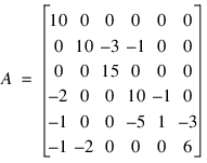
As an example, consider the following matrix:
Let:
x1T = (1, 2, 3, 4, 5, 6)
so that:
x1 = (10, 7, 45, 33, –34, 31)T,
and let:
x2T = (5, 10, 15, 15, 10, 5)
so that:
Ax2 = (50, 40, 225, 130, –85, 5)T
In this example we factor A using SP_LUFAC, and compute solutions to the systems Ax1 = b1 and Ax2 = b2 using the computed factor as input to SP_LUSOL.
; Define the sparse matrix A using coordinate storage format.
A = replicate(!F_sp_elem, 15)
a(*).row = [0, 1, 1, 1, 2, 3, 3, 3, 4, 4, 4, 4, 5, 5, 5]
a(*).col = [0, 1, 2, 3, 2, 0, 3, 4, 0, 3, 4, 5, 0, 1, 5]
a(*).val = [10, 10, -3, -1, 15, -2, 10, -1, -1, -5, $
1, -3, -1, -2, 6]
; Define the right-hand sides.
b1 = [10, 7, 45, 33, -34, 31]
b2 = [50, 40, 225, 130, -85, 5]
; Compute the LU factorization.
factor = SP_LUFAC(a, 6)
; Call SP_LUSOL with factor and b1, then print result and the sum
; of the residuals.
x1 = SP_LUSOL(b1, factor_coord = factor)
PM, x1
; PV-WAVE prints the following:
; 1.0000000
; 2.0000000
; 3.0000000
; 4.0000000
; 5.0000000
; 6.0000000
PM, TOTAL(ABS(SP_MVMUL(6, 6, a, x1) - b1))
; PV-WAVE prints: 8.8817842e-16
; Call SP_LUSOL with factor and b2, then print out result and the
; sum of the residuals.
x2 = SP_LUSOL(b2, factor_coord = factor)
PM, x2
; PV-WAVE prints the following:
; 5.0000000
; 10.000000
; 15.000000
; 15.000000
; 10.000000
; 5.0000000
PM, TOTAL(ABS(SP_MVMUL(6, 6, a, x2) - b2))
; PV-WAVE prints: 1.4210855e-14
See Also
Version 2017.0
Copyright © 2017, Rogue Wave Software, Inc. All Rights Reserved.