SP_PDFAC Function (PV-WAVE Advantage)
Computes a factorization of a sparse symmetric positive definite system of linear equations Ax = b.
Usage
result = SP_PDFAC(a, n_rows)
Input Parameters
a—Sparse matrix stored as an array of structures containing non-zeros in lower triangle of the coefficient matrix A(i,j). See the chapter introduction for a description of structures used for sparse matrices.
n_rows—The number of rows in a.
Returned Value
result—The factorization of Ax = b.
Input Keywords
Multifrontal—If present and nonzero, perform the numeric factorization using a multifrontal technique. By default a standard factorization is computed based on a sparse compressed storage scheme
Csc_col—Accept the coefficient matrix in compressed sparse column (CSC) format. The keywords Csc_col, Csc_row, and Csc_val must be used together.
Csc_row—Accept the coefficient matrix in compressed sparse column (CSC) format. See the chapter introduction for a discussion of this storage scheme. The keywords Csc_col, Csc_row, and Csc_val must be used together.
Csc_val—Accept the coefficient matrix in compressed sparse column (CSC) format. See the chapter introduction for a discussion of this storage scheme. The keywords Csc_col, Csc_row, and Csc_val must be used together.
Output Keywords
Sm_diag—The smallest diagonal element that occurred during the numeric factorization.
Lg_diag—The largest diagonal element that occurred during the numeric factorization.
N_nonzero—Specifies a named variable into which the total number of non-zeros in the factor is stored.
Discussion
The function SP_PDFAC computes a factorization of a sparse symmetric positive definite coefficient matrix A. In this function’s default usage, a symbolic factorization of a permutation of the coefficient matrix is computed first. Then a numerical factorization is performed.
The symbolic factorization step of the computation consists of determining a minimum degree ordering and then setting up a sparse data structure for the Cholesky factor, L. This step only requires the “pattern” of the sparse coefficient matrix, that is, the locations of the non-zero elements but not any of the elements themselves.
The numerical factorization can be carried out in one of two ways. By default, the standard factorization is performed based on a sparse compressed storage scheme. This is fully described in George and Liu (1981). Optionally, a multifrontal technique can be used. The multifrontal method requires more storage but will be faster in certain cases. The multifrontal factorization is based on the routines in Liu (1987). For a detailed description of this method, see Liu (1990), also Duff and Reid (1983, 1984), Ashcraft (1987), Ashcraft, et al. (1987), and Liu (1986, 1989).
If an application requires that several linear systems be solved where the coefficient matrix is the same but the right-hand sides change, SP_PDFAC can be used to precompute the Cholesky factor. Then the keyword Factor can be used in SP_PDSOL to efficiently solve all subsequent systems.
Given numeric factorization, x is obtained by the following calculations:
Ly1 = Pb
LTy2 = y1
x = PTy2
The permutation information, P, is carried in the numeric factor structure.
Example 1
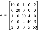
As an example consider the 5 × 5 coefficient matrix:
Let x1T = (5, 4, 3, 2, 1) so that Ax1 = (55, 83, 103, 97, 82)T. Let x2T = (1, 2, 3, 4, 5) so that Ax2 = (23, 55, 107, 197, 278)T. The number of non-zeros in the lower triangle of A is nz = 10. The sparse coordinate form for the lower triangle is given by:
row | 0 | 1 | 2 | 2 | 3 | 3 | 4 | 4 | 4 | 4 |
col | 0 | 1 | 0 | 2 | 2 | 3 | 0 | 1 | 3 | 4 |
val | 10 | 20 | 1 | 30 | 4 | 40 | 2 | 3 | 5 | 50 |
Since this representation is not unique, an equivalent form would be:
row | 3 | 4 | 4 | 4 | 0 | 1 | 2 | 2 | 3 | 4 |
col | 3 | 0 | 1 | 3 | 0 | 1 | 0 | 2 | 2 | 4 |
val | 40 | 2 | 3 | 5 | 10 | 20 | 1 | 30 | 4 | 50 |
A = REPLICATE(!F_sp_elem, 10)
a(*).row = [0, 1, 2, 2, 3, 3, 4, 4, 4, 4]
a(*).col = [0, 1, 0, 2, 2, 3, 0, 1, 3, 4]
a(*).val = [10, 20, 1, 30, 4, 40, 2, 3, 5, 50]
b1 = [55, 83, 103, 97, 82]
b2 = [23, 55, 107, 197, 278]
factor = SP_PDFAC(a, 5)
x1 = SP_PDSOL(b1, FACTOR = factor)
PM, x1 ; PV-WAVE prints the following:
; 5.0000000
; 4.0000000
; 3.0000000
; 2.0000000
; 1.0000000
x2 = SP_PDSOL(b2, FACTOR = factor)
PM, x2 ; PV-WAVE prints the following:
; 1.0000000
; 2.0000000
; 3.0000000
; 4.0000000
; 5.0000000
See Also
Version 2017.0
Copyright © 2017, Rogue Wave Software, Inc. All Rights Reserved.