SP_GMRES Function (PV-WAVE Advantage)
Solves a linear system Ax = b using the restarted generalized minimum residual (GMRES) method.
Usage
result = SP_GMRES(amultp, b)
Input Parameters
amultp—Scalar string specifying a user supplied function that computes
z = Ap. The function accepts the argument p, and returns the vector Ap.
b—One-dimensional matrix containing the right-hand side.
Returned Value
result—A one-dimensional array containing the solution of the linear system Ax = b.
Input Keywords
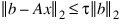
Tolerance—The algorithm attempts to generate x such that:
where t = Tolerance. Default: Tolerance = SQRT(machine precision).
Precond—Scalar sting specifying a user supplied function which sets z = M–1r, where M is the preconditioning matrix.
Max_krylov—The maximum Krylov subspace dimension, that is, the maximum allowable number of GMRES iterations allowed before restarting. Default: Max_krylov= Minimum(N_ELEMENTS(b), 20).
Hh_reorth—If present and nonzero, perform orthogonalization by Householder transformations, replacing the Gram-Schmidt process.
Double—If present and nonzero, double precision is used.
Input/Output Keywords
Itmax—Initially set to the maximum number of GMRES iterations allowed. On exit, the number of iterations used is returned. Default: Itmax= 1000
Discussion
The function SP_GMRES, based on the FORTRAN subroutine GMRESD by H. F. Walker, solves the linear system Ax = b using the GMRES method. This method is described in detail by Saad and Schultz (1986) and Walker (1988).
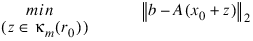
The GMRES method begins with an approximate solution x0 and an initial residual r0 = b – Ax0. At iteration m, a correction zm is determined in the Krylov subspace:
κm(v) = span(v, Av, ..., Am–1v)
v = r0 which solves the least squares problem:
Then at iteration m, xm = x0 + zm.
Orthogonalization by Householder transformations requires less storage but more arithmetic than Gram-Schmidt. However, Walker (1988) reports numerical experiments which suggest the Householder approach is more stable, especially as the limits of residual reduction are reached.
Example 1
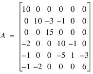
In this example, the solution to a linear system is found. The coefficient matrix is stored in coordinate format. Consider the following matrix:
Let xT = (1, 2, 3, 4, 5, 6) so that Ax = (10, 7, 45, 33, –34, 31)T. The number of nonzeros in A is 15.
; This function uses SP_MVMUL to multiply a sparse matrix stored
; in coordinate storage mode and a vector. The common block
; holds the sparse matrix.
FUNCTION Amultp, p
COMMON Gmres_ex1, nrows, ncols, a
RETURN, SP_MVMUL(nrows, ncols, a, p)
END
; This procedure defines the sparse matrix A stored in coordinate
; storage mode, and then calls SP_GMRES to compute the solution
; to Ax = b.
PRO Gmres1
COMMON Gmres_ex1, nrows, ncols, a
A = replicate(!F_sp_elem, 15)
a(*).row = [0, 1, 1, 1, 2, 3, 3, 3, 4, 4, 4, 4, 5, 5, 5]
a(*).col = [0, 1, 2, 3, 2, 0, 3, 4, 0, 3, 4, 5, 0, 1, 5]
a(*).val = [10, 10, -3, -1, 15, -2, 10, -1, -1, -5, $
1, -3, -1, -2, 6]
nrows = 6
ncols = 6
b = [10, 7, 45, 33, -34, 31]
; Itmax is input/output.
itmax = 10
x = SP_GMRES('amultp', b, Itmax = itmax) PM, x, title = 'Solution to Ax = b'
PM, itmax, title = 'Number of iterations'
END
; Output of this procedure:
; Solution to Ax = b
; 1.0000000
; 2.0000000
; 3.0000000
; 4.0000000
; 5.0000000
; 6.0000000
; Number of iterations
; 6
See Also
Version 2017.0
Copyright © 2017, Rogue Wave Software, Inc. All Rights Reserved.