GENEIG Procedure (PV-WAVE Advantage)
Computes the generalized eigenexpansion of a system Ax = λBx.
Usage
GENEIG, a, b, alpha, beta
Input Parameters
a—Two-dimensional array of size n-by-n containing coefficient matrix A.
b—Two-dimensional array of size n-by-n containing coefficient matrix B.
Output Parameters
alpha—One-dimensional array of size n containing scalars αi. If βi ≠ 0, λi = αi /βi for i = 0, ..., n – 1 are the eigenvalues of the system.
beta—One-dimensional array of size n.
Input Keywords
Double—If present and nonzero, double precision is used.
Output Keywords
Vectors—Named variable into which a two-dimensional array of size n-by-n containing eigenvectors of the problem is stored. Each vector is normalized to have Euclidean length equal to one.
Discussion
The function GENEIG uses the QZ algorithm to compute the eigenvalues and eigenvectors of the generalized eigensystem Ax = λBx, where A and B are matrices of order n. The eigenvalues for this problem can be infinite, so α and β are returned instead of λ. If β is nonzero, λ = α/β.
The first step of the QZ algorithm is to simultaneously reduce A to upper-Hessenberg form and B to upper-triangular form. Then, orthogonal transformations are used to reduce A to quasi-upper-triangular form while keeping B upper triangular. The generalized eigenvalues and eigenvectors for the reduced problem are then computed.
The function GENEIG is based on the QZ algorithm due to Moler and Stewart (1973), as implemented by the EISPACK routines QZHES, QZIT and QZVAL; see Garbow et al. (1977).
Example 1
In this example, the eigenvalue, λ, of system Ax = λBx is computed, where:
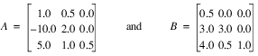
a = TRANSPOSE([[1.0, 0.5, 0.0], [-10.0, 2.0, 0.0], $
[5.0, 1.0, 0.5]])
b = TRANSPOSE([[0.5, 0.0, 0.0], [3.0, 3.0, 0.0], $
[4.0, 0.5, 1.0]])
; Compute eigenvalues
GENEIG, a, b, alpha, beta
; Print eigenvalues
PM, alpha/beta, Title = 'Eigenvalues'
; PV-WAVE prints the following:
; Eigenvalues
; ( 0.833334, 1.99304)
; ( 0.833333, -1.99304)
; ( 0.500000, 0.00000)
Example 2
This example finds the eigenvalues and eigenvectors of the same eigensystem given in the last example.
a = TRANSPOSE([[1.0, 0.5, 0.0], [-10.0, 2.0, 0.0], $
[5.0, 1.0, 0.5]])
b = TRANSPOSE([[0.5, 0.0, 0.0], [3.0, 3.0, 0.0], $
[4.0, 0.5, 1.0]])
; Compute eigenvalues
GENEIG, a, b, alpha, beta, Vectors = vectors
; Print eigenvalues
PM, alpha/beta, Title = 'Eigenvalues'
; PV-WAVE prints the following:
; Eigenvalues
; ( 0.833332, 1.99304)
; ( 0.833332, -1.99304)
; ( 0.500000, -0.00000)
; Print eigenvectors
PM, vectors, Title = 'Eigenvectors'
; PV-WAVE prints the following:
; Eigenvectors
; ( -0.197112, 0.149911)( -0.197112, -0.149911)
; ( -1.53306e-08, 0.00000)
; ( -0.0688163, -0.567750)( -0.0688163, 0.567750)
; ( -4.75248e-07, 0.00000)
; ( 0.782047, 0.00000)( 0.782047, 0.00000)
; ( 1.00000, 0.00000)
Example 3
In this example, the eigenvalue, λ, of system Ax = λBx is solved, where:
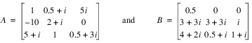
a = TRANSPOSE([$
[COMPLEX(1.0, 0.0), COMPLEX(0.5, 1.0), COMPLEX(0.0, 5.0)], $
[COMPLEX(-10.0, 0.0), COMPLEX(2.0, 1.0), COMPLEX(0.0, 0.0)], $
[COMPLEX(5.0, 1.0), COMPLEX(1.0, 0.0), COMPLEX(0.5, 3.0)]])
b = TRANSPOSE([$
[COMPLEX(0.5, 0.0), COMPLEX(0.0, 0.0), COMPLEX(0.0, 0.0)], $
[COMPLEX(3.0, 3.0), COMPLEX(3.0, 3.0), COMPLEX(0.0, 1.0)], $
[COMPLEX(4.0, 2.0), COMPLEX(0.5, 1.0), COMPLEX(1.0, 1.0)]])
; Compute eigenvalues
GENEIG, a, b, alpha, beta
; Print eigenvalues
PM, alpha/beta, Title = 'Eigenvalues'
; PV-WAVE prints the following:
; Eigenvalues
; ( -8.18016, -25.3799)
; ( 2.18006, 0.609113)
; ( 0.120108, -0.389223)
Example 4
This example finds the eigenvalues and eigenvectors of the same eigensystem given in the last example.
a = TRANSPOSE([$
[COMPLEX(1.0, 0.0), COMPLEX(0.5, 1.0), COMPLEX(0.0, 5.0)], $
[COMPLEX(-10.0, 0.0), COMPLEX(2.0, 1.0), COMPLEX(0.0, 0.0)], $
[COMPLEX(5.0, 1.0), COMPLEX(1.0, 0.0), COMPLEX(0.5, 3.0)]])
b = TRANSPOSE([$
[COMPLEX(0.5, 0.0), COMPLEX(0.0,0.0), COMPLEX(0.0, 0.0)], $
[COMPLEX(3.0,3.0), COMPLEX(3.0,3.0), COMPLEX(0.0, 1.0)], $
[COMPLEX(4.0, 2.0), COMPLEX(0.5, 1.0), COMPLEX(1.0, 1.0)]])
; Compute eigenvalues
GENEIG, a, b, alpha, beta, Vectors = vectors
; Print eigenvalues
PM, alpha/beta, Title = 'Eigenvalues'
; PV-WAVE prints the following:
; Eigenvalues
; ( -8.18018, -25.3799)
; ( 2.18006, 0.609112)
; ( 0.120109, -0.389223)
; Print eigenvecters
PM, vectors, Title = 'Eigenvectors'
; PV-WAVE prints the following:
; Eigenvectors
; ( -0.326709, -0.124509)( -0.300678, -0.244401)
; ( 0.0370698, 0.151778)
; ( 0.176670, 0.00537758)( 0.895923, 0.00000)
; ( 0.957678, 0.00000)
; ( 0.920064, 0.00000)( -0.201900, 0.0801192)
; ( -0.221511, 0.0968290)
Version 2017.0
Copyright © 2017, Rogue Wave Software, Inc. All Rights Reserved.