REGRESSORS Function (PV-WAVE Advantage)
Generates regressors for a general linear model.
Usage
result = REGRESSORS(x, n_class, n_continuous)
Input Parameters
x—Two-dimensional array containing the data. The columns must be ordered such that the first n_class columns contain the class variables and the next n_continuous columns contain the continuous variables. (Exception: See keyword Class_Columns.)
n_class—Number of classification variables.
n_continuous—Number of continuous variables.
Returned Value
result—A two-dimensional array containing the regressor variables generated from x.
Input Keywords
Double—If present and nonzero, double precision is used.
Class_Columns—One-dimensional array of length n_class containing the column numbers of x that are the classification variables. The remaining n_continuous variables are assumed to correspond to the columns of x in the range 0, ..., n_class – 1 that are not listed in Class_Columns. Default: Class_Columns = [0, 1, ..., n_class – 1]
Order—Order of the model. Model order can be specified as 1 or 2. Use keyword Indices_Effects to specify more complicated models. The keywords Var_Effects and Indices_Effects must be used together. Default: Order = 1
Var_Effects—One-dimensional array containing the number of variables associated with each effect in the model. The keywords Var_Effects and Indices_Effects must be used together.
Indices_Effects—One-dimensional array of length Var_Effects (0) + Var_Effects (1) + ... Var_Effects (N_ELEMENTS (Var_Effects) – 1). The first Var_Effects(0) elements give the column numbers of x for each variable in the first effect. The next Var_Effects(1) elements give the column numbers for each variable in the second effect. The last Var_Effects (N_ELEMENTS (Var_Effects) – 1) elements give the column numbers for each variable in the last effect. Keywords Var_Effects and Indices_Effects must be used together.
Dummy_Method—Dummy variable option. Indicator variables are defined for each class variable as described in the Discussion section. Dummy variables are then generated from the n indicator variables in one of the following three ways:

(Default)—The
n indicator variables are the dummy variables.
1—Dummies are the first
n – 1 indicator variables.
2—The
n – 1 dummies are defined in terms of the indicator variables so that for balanced data, the usual summation restrictions are imposed on the regression coefficients.
Discussion
Function REGRESSORS generates regressors for a general linear model from a data matrix. The data matrix can contain classification variables as well as continuous variables. Regressors for effects composed solely of continuous variables are generated as powers and crossproducts. Consider a data matrix containing continuous variables as Columns 3 and 4. The effect indices (3, 3) generate a regressor whose ith value is the square of the ith value in Column 3. The effect indices (3, 4) generates a regressor whose ith value is the product of the ith value in Column 3 with the ith value in Column 4.
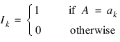
Regressors for an effect (source of variation) composed of a single classification variable are generated using indicator variables. Let the classification variable A take on values a1, a2, ..., an. From this classification variable, REGRESSORS creates n indicator variables. For k = 1, 2, ..., n:
For each classification variable, another set of variables is created from the indicator variables. These new variables are called dummy variables. Dummy variables are generated from the indicator variables in one of three manners:
1. The dummies are the n indicator variables. (Default method)
2. The dummies are the first n – 1 indicator variables. (Dummy_Method = 1)
3. The n – 1 dummies are defined in terms of the indicator variables so that for balanced data, the usual summation restrictions are imposed on the regression coefficients. (Dummy_Method = 2)
For the default case, the dummy variables are Ak = Ik (k = 1, 2, ..., n). For Dummy_Method = 1, the dummy variables are Ak = Ik (k = 1, 2, ..., n – 1). For Dummy_Method = 2, the dummy variables are Ak = Ik – In (k = 1, 2, ..., n – 1). The regressors generated for an effect composed of a single-classification variable are the associated dummy variables.
Let mj be the number of dummies generated for the jth classification variable. Suppose there are two classification variables A and B with dummies:
The regressors generated for an effect composed of two classification variables A and B are:
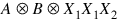
More generally, the regressors generated for an effect composed of several classification variables and several continuous variables are given by the Kronecker products of variables, where the order of the variables is specified in Indices_Effects. Consider a data matrix containing classification variables in Columns 0 and 1 and continuous variables in Columns 2 and 3. Label these four columns A, B, X1, and X2. The regressors generated by the effect indices (0, 1, 2, 2, 3) are:
Remarks
Let the data matrix x = (A, B, X1), where A and B are classification variables and X1 is a continuous variable. The model containing the effects A, B, AB, X1, AX1, BX1, and ABX1 is specified as follows (use optional keyword Indices_Effects):
n_class = 2
n_continuous = 1
Var_Effects = [1, 1, 2, 1, 2, 2, 3]
Indices_Effects = [0, 1, 0, 1, 2, 0, 2, 1, 2, 0, 1, 2]
For this model, suppose that variable A has two levels, A1 and A2, and that variable B has three levels, B1, B2, and B3. For each Dummy_Method option, the regressors in their order of appearance in REGRESSORS are given below:
(Default)—
A1,
A2,
B1,
B2,
B3,
A1 B1,
A1 B2,
A1 B3,
A2 B1,
A2 B2,
A2 B3,
X1,
A1 X1,
A2 X1,
B1 X1,
B2 X1,
B3 X1,
A1 B1 X1,
A1 B2 X1,
A1 B3 X1,
A2 B1 X1,
A2 B2 X1,
A2 B3 X11—
A1,
B1,
B2,
A1 B1,
A1 B2,
X1,
A1 X1,
B1 X1,
B2 X1, –
A1 B1 X1,
A1 B2 X1 2—
A1 –
A2,
B1 –
B3,
B2 –
B3, (
A1 –
A2) (
B1 –
B2), (
A1 –
A2) (
B2 –
B3),
X1, (
A1 –
A2)
X1, (
B1 –
B3)
X1, (
B2 –
B3)
X1, (
A1 –
A2) (
B1 –
B2)
X1, (
A1 –
A2) (
B2 –
B3)
X1Within a group of regressors corresponding to an interaction effect, the indicator variables composing the regressors vary most rapidly for the last classification variable, next most rapidly for the next to last classification variable, etc.
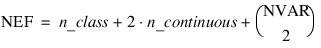
By default, REGRESSORS internally generates values for Var_Effects and Indices_Effects, which correspond to a first order model with NEF = n_continuous + n_class. The variables then are used to create the regressor variables. The effects are ordered such that the first effect corresponds to the first column of x, the second effect corresponds to the second column of x, etc. A second order model corresponding to the columns (variables) of x is generated if Order with Order = 2 is specified.
There are:
effects, where NVAR = n_continuous + n_class. The first NVAR effects correspond to the columns of x, such that the first effect corresponds to the first column of x, the second effect corresponds to the second column of x, ..., the NVARth effect corresponds to the NVARth column of x (i.e., x (NVAR – 1)). The next n_continuous effects correspond to squares of the continuous variables. The last:
effects correspond to the two-variable interactions.
Let the data matrix
x = (
A,
B,
X1), where
A and
B are classification variables and
X1 is a continuous variable. The effects generated and order of appearance is
A,
B,
X1,
X21,
AB,
AX1,
BX1.
Let the data matrix
x = (
A,
X1,
X2), where
A is a classification variable and
X1 and
X2 are continuous variables. The effects generated and order of appearance is
A,
X1,
X2,
X21,
X22,
AX1,
AX2,
X1X2.
Let the data matrix
x = (
X1,
A,
X2) (see
Class_Columns), where
A is a classification variable and
X1 and
X2 are continuous variables. The effects generated and order of appearance is
X1,
A,
X2,
X21,
X22,
X1A,
X1X2,
AX2.
Higher-order and more complicated models can be specified using Indices_Effects.
Example 1
In the following example, there are two classification variables, A and B, with two and three values, respectively. Regressors for a one-way model (the default model order) are generated using the ALL dummy method (the default dummy method). The five regressors generated are A1, A2, B1, B2, B3.
; Define some labels for printing later and enter the data.
labels = ['A1', 'A2', 'B1', 'B2', 'B3']
RM, x, 6, 2
row 0: 10 5
row 1: 20 15
row 2: 20 10
row 3: 10 10
row 4: 10 15
row 5: 20 5
; Call REGRESSORS.
reg = REGRESSORS(x, 2, 0)
; Print the results.
PM, labels, reg, Format = '(5a8, /, 6(5f8.1, /))'
This results in the following output:
A1 A2 B1 B2 B3
1.0 0.0 1.0 0.0 0.0
0.0 1.0 0.0 0.0 1.0
0.0 1.0 0.0 1.0 0.0
1.0 0.0 0.0 1.0 0.0
1.0 0.0 0.0 0.0 1.0
0.0 1.0 1.0 0.0 0.0
Example 2
In this example, a two-way analysis of covariance model containing all the interaction terms is fit. First, REGRESSORS is called to produce a matrix of regressors, reg, from the data x. The regressors, generated using Dummy_Method = 1, are the model whose mean function is:
μ + αi + βj + γij + δ xij + ζixij + η j xij + θijxij i = 1, 2; j = 1, 2, 3
where α2 = β3 = γ21 = γ22 = γ23 = ζ2 = η3 = θ21 = θ22 = θ23 = 0.
; Define some labels to use in printing the results.
labels = ['Alpha1', 'Beta1', 'Beta2', 'Gamma11', 'Gamma12', $
'Delta', 'Zeta1', 'Eta1', 'Eta2', 'Theta11', 'Theta12']
x = transpose([ [1.0, 1.0, 1.11], [1.0, 1.0, 2.22], $
[1.0, 1.0, 3.33], [1.0, 2.0, 1.11], [1.0, 2.0, 2.22], $
[1.0, 2.0, 3.33], [1.0, 3.0, 1.11], [1.0, 3.0, 2.22], $
[1.0, 3.0, 3.33], [2.0, 1.0, 1.11], [2.0, 1.0, 2.22], $
[2.0, 1.0, 3.33], [2.0, 2.0, 1.11], [2.0, 2.0, 2.22], $
[2.0, 2.0, 3.33], [2.0, 3.0, 1.11], [2.0, 3.0, 2.22], $
[2.0, 3.0, 3.33]])
Var_Effects = [1, 1, 2, 1, 2, 2, 3]
Indices_Effects = [0, 1, 0, 1, 2, 0, 2, 1, 2, 0, 1, 2]
; Call REGRESSORS.
reg = REGRESSORS(x, 2, 1, Dummy_Method = 1, $
Var_Effects = var_effects, Indices_Effects = indices_effects)
PM, labels(0:5), reg(*, 0:5), Format = '(6a9, /, 18(6f9.2, /))'
; Output the results.
; Alpha1 Beta1 Beta2 Gamma11 Gamma12 Delta
; 1.0 1.0 0.0 1.0 0.0 1.1
; 1.00 1.00 0.00 1.00 0.00 2.22
; 1.00 1.00 0.00 1.00 0.00 3.33
; 1.00 0.00 1.00 0.00 1.00 1.11
; 1.00 0.00 1.00 0.00 1.00 2.22
; 1.00 0.00 1.00 0.00 1.00 3.33
; 1.00 0.00 0.00 0.00 0.00 1.11
; 1.00 0.00 0.00 0.00 0.00 2.22
; 1.00 0.00 0.00 0.00 0.00 3.33
; 0.00 1.00 0.00 0.00 0.00 1.11
; 0.00 1.00 0.00 0.00 0.00 2.22
; 0.00 1.00 0.00 0.00 0.00 3.33
; 0.00 0.00 1.00 0.00 0.00 1.11
; 0.00 0.00 1.00 0.00 0.00 2.22
; 0.00 0.00 1.00 0.00 0.00 3.33
; 0.00 0.00 0.00 0.00 0.00 1.11
; 0.00 0.00 0.00 0.00 0.00 2.22
; 0.00 0.00 0.00 0.00 0.00 3.33
PM, labels(6:10), reg(*, 6:10), Format = '(5a9, /, 18(5f9.2, /))'
; Output the results:
; Zeta1 Eta1 Eta2 Theta11 Theta12
; 1.1 1.1 0.0 1.1 0.0
; 2.22 2.22 0.00 2.22 0.00
; 3.33 3.33 0.00 3.33 0.00
; 1.11 0.00 1.11 0.00 1.11
; 2.22 0.00 2.22 0.00 2.22
; 3.33 0.00 3.33 0.00 3.33
; 1.11 0.00 0.00 0.00 0.00
; 2.22 0.00 0.00 0.00 0.00
; 3.33 0.00 0.00 0.00 0.00
; 0.00 1.11 0.00 0.00 0.00
; 0.00 2.22 0.00 0.00 0.00
; 0.00 3.33 0.00 0.00 0.00
; 0.00 0.00 1.11 0.00 0.00
; 0.00 0.00 2.22 0.00 0.00
; 0.00 0.00 3.33 0.00 0.00
; 0.00 0.00 0.00 0.00 0.00
; 0.00 0.00 0.00 0.00 0.00
; 0.00 0.00 0.00 0.00 0.00
Version 2017.0
Copyright © 2017, Rogue Wave Software, Inc. All Rights Reserved.