HYPOTH_TEST Function (PV-WAVE Advantage)
Performs tests for a multivariate general linear hypothesis HβU = G given the hypothesis sums of squares and crossproducts matrix SH.
Usage
result = HYPOTH_TEST(info_v, dfh, scph)
Input Parameters
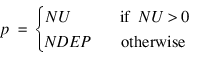
info_v—One-dimensional array of type BYTE containing information about the regression fit. See function MULTIREGRESS.
dfh—Degrees of freedom for the sums of squares and crossproducts matrix.
scph—Two-dimensional array of size nu by nu containing SH, the sums of squares and crossproducts attributable to the hypothesis.
Returned Value
result—The p-value corresponding to Wilks’ lambda test.
Input Keywords
Double—If present and nonzero, double precision is used.
U—Two-dimensional array of size n_dependent by nu containing the U matrix for the test HpβU = Gp where nu is the number of linear combinations of the dependent variables to be considered. The value nu must be greater than 0 and less than or equal to n_dependent. Default: nu = n_dependent and U is the identity matrix
Output Keywords
Wilk_Lambda—Named variable into which the one-dimensional array containing the Wilk’s lamda and p-value is stored.
Roy_Max_Root—Named variable into which the one-dimensional array containing the Roy’s maximum root criterion and p-value is stored.
Hotelling_Trace—Named variable into which the one-dimensional array containing the Hotelling’s trace and p-value is stored.
Pillai_Trace—Named variable into which the one-dimensional array containing the Pillai’s trace and p-value is stored.
Discussion
HYPOTH_TEST computes test statistics and p-values for the general linear hypothesis HβU = G for the multivariate general linear model.
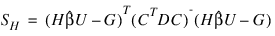
The hypothesis sum of squares and crossproducts matrix input in scph is:
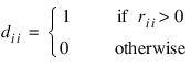
where C is a solution to RTC = H and where D is a diagonal matrix with diagonal elements:
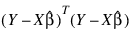
Error sum of squares and crossproducts matrix for model Y = Xβ + ε is:
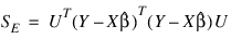
which is input in MULTIREGRESS. The error sum of squares and crossproducts matrix for the hypothesis HβU = G computed by HYPOTH_TEST is:
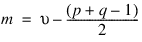
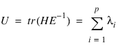
Let p equal the order of the matrices SE and SH, i.e.:
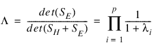
Let q (stored in dfh) be the degrees of freedom for the hypothesis. Let v (input in info_v) be the degrees of freedom for error. Function HYPOTH_TEST computed three test statistics based on eigenvalues λi (i = 1, 2, ... p) of the generalized eigenvalue problem SHx = λSEx. These test statistics are as follows:
Wilk’s lambda:
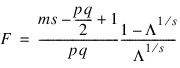
The associated p-value is based on an approximation discussed by Rao (1973, p. 556). The statistic:
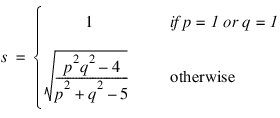
has an approximate F distribution with pq and ms – pq/2 + 1 numerator and denominator degrees of freedom, respectively, where:
and:
The F test is exact if min (p, q) ≤ 2 (Kshirsagar, 1972, Theorem 4, p. 2994300).
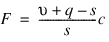
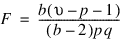
Roy’s maximum root:
c = max λ i over all i
where c is output as value = Roy_Max_Root(0). The p-value is based on the approximation:
where s = max (p, q) has an approximate F distribution with s and υ + q − s numerator and denominator degrees of freedom, respectively. The F test is exact if s = 1; the p-value is also exact. In general, the value output in p_value = Roy_Max_Root(1) is lower bound on the actual p-value.
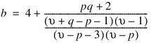
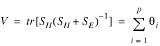
Hotelling’s trace:
U is output as value = Hotelling_Trace(0). The p-value is based on the approximation of McKeon (1974) that supersedes the approximation of Hughes and Saw (1972). McKeon’s approximation is also discussed by Seber (1984, p. 39). For:
the p-value is based on the result that:
has an approximate F distribution with pq and b degrees of freedom. The test is exact if min (p, q) = 1. For υ ≤ p + 1, the approximation is not valid, and p_value = Hotelling_Trace(1) is set to NaN.
These three test statistics are valid when SE is positive definite. A necessary condition for SE to be positive definite is υ ≥ p. If SE is not positive definite, a warning error message is issued, and both value and p_value are set to NaN.
Because the requirement υ ≥ p can be a serious drawback, HYPOTH_TEST computes a fourth test statistic based on eigenvalues θi (i = 1, 2, ..., p) of the generalized eigenvalue problem SHw = θ(SH + SE) w. This test statistic requires a less restrictive assumption—SH + SE is positive definite. A necessary condition for SH + SE to be positive definite is υ + q ≥ p. If SE is positive definite, HYPOTH_TEST avoids the computation of the generalized eigenvalue problem from scratch. In this case, the eigenvalues θi are obtained from λi by:
The fourth test statistic is as follows:
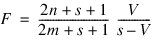
Pillai’s trace:
V is output as value = Pillai_Trace(0). The p-value is based on an approximation discussed by Pillai (1985). The statistic:
has an approximate F distribution with s(2m + s + 1) and s(2n + s + 1) numerator and denominator degrees of freedom, respectively, where:
s = min (p, q)
m = 1/2(|p - q| – 1)
n = 1/2(υ - p – 1)
The F test is exact if min (p, q) = 1.
Example 1
The data for this example are from Maindonald (1984, p. 20310204). A multivariate regression model containing two dependent variables and three independent variables is fit using function MULTIREGRESS and the results stored in info_v. The sum of squares and crossproducts matrix, scph, is then computed using HYPOYH_SCPH for the test that the third independent variable is in the model (determined by specification of h). Finally, function HYPOTH_TEST is used to compute the p-value for the test statistic (Wilk’s lambda).
x = TRANSPOSE([[7.0, 5.0, 6.0], [2.0, -1.0, 6.0], $
[7.0, 3.0, 5.0], [-3.0, 1.0, 4.0], [2.0, -1.0, 0.0], $
[2.0, 1.0, 7.0], [-3.0, -1.0, 3.0], [2.0, 1.0, 1.0], $
[2.0, 1.0, 4.0]])
y = TRANSPOSE([[7.0, 1.0], [-5.0, 4.0], [6.0, 10.0], $
[5.0, 5.0], [5.0, -2.0], [-2.0, 4.0], [0.0, -6.0], $
[8.0, 2.0], [3.0, 0.0]])
h = FLTARR(1, 4)
h(*) = 0
h(0, 3) = 1.0
coefs = MULTIREGRESS(x, y, Predict_Info = p)
scph = HYPOTH_SCPH(p, h, Dfh = dfh)
pvalue = HYPOTH_TEST(p, dfh, scph)
PM, pvalue, format = '(F10.6)', Title = 'P-value'
; PV-WAVE prints the following:
; P-value
; 0.000010
Example 2
This example is the same as the first example, but more statistics are computed. Also, the U matrix, U, is explicitly specified as the identity matrix (which is the same default configuration of U).
x = TRANSPOSE([[7.0, 5.0, 6.0], [2.0, -1.0, 6.0], $
[7.0, 3.0, 5.0], [-3.0, 1.0, 4.0], [2.0, -1.0, 0.0], $
[2.0, 1.0, 7.0], [-3.0, -1.0, 3.0], [2.0, 1.0, 1.0], $
[2.0, 1.0, 4.0]])
y = TRANSPOSE([[7.0, 1.0], [-5.0, 4.0], [6.0, 10.0], $
[5.0, 5.0], [5.0, -2.0], [-2.0, 4.0], [0.0, -6.0], $
[8.0, 2.0], [3.0, 0.0]])
h = FLTARR(1, 4)
h(*) = 0
h(0, 3) = 1.0
u = [[1, 0], [0, 1]]
coefs = MULTIREGRESS(x, y, Predict_Info = p)
scph = HYPOTH_SCPH(p, h, Dfh = dfh)
pvalue = HYPOTH_TEST(p, dfh, scph, U = u, $
Wilk_Lambda = wilk_lambda, Roy_Max_Root = roy_max_root, $
Hotelling_Trace = hotelling_trace, $
Pillai_Trace = pillai_trace)
PRINT, 'Wilk value = ', wilk_lambda(0), ' p-value =', $
wilk_lambda(1)
; PV-WAVE prints: Wilk value = 0.00314861 p-value = 9.89437e-06
PRINT, 'Roy value = ', roy_max_root(0), ' p-value =', $
roy_max_root(1)
; PV-WAVE prints: Roy value = 316.601 p-value = 9.89437e-06
PRINT, 'Hotelling value = ', hotelling_trace(0), ' p-value =', $
hotelling_trace(1)
; PV-WAVE prints: Hotelling value = 316.601 p-value = 9.89437e-06
PRINT, 'Pillai value = ', pillai_trace(0), ' p-value =', $
pillai_trace(1)
; PV-WAVE prints: Pillai value = 0.996851 p-value = 9.89437e-06
Warning Errors
STAT_SINGULAR_1—“u”*“scpe”*“u” is singular. Only Pillai’s trace can be computed. Other statistics are set to NaN.
Fatal Errors
STAT_NO_STAT_1—“scpe” + “scph” is singular. No tests can be computed.
STAT_NO_STAT_2—No statistics can be computed. Iterations for eigenvalues for the generalized eigenvalue problem “scph”*x = (lambda)*(“scph”+“scpe”)*x failed to converge.
STAT_NO_STAT_3—No statistics can be computed. Iterations for eigenvalues for the generalized eigenvalue problem “scph”*x = (lambda)*(“scph”+“u”*“scpe”*“u”)*x failed to converge.
STAT_SINGULAR_2—“u”*“scpe”*“u” + “scph” is singular. No tests can be computed.
STAT_SINGULAR_TRI_MATRIX—The input triangular matrix is singular. The index of the first zero diagonal element is equal to #.
Version 2017.0
Copyright © 2017, Rogue Wave Software, Inc. All Rights Reserved.