ODEBV Function (PV-WAVE Advantage)
Solves a general system of ordinary differential equations dy/dx = f(x,y), with boundary conditions h(y(a), y(b)) = 0.
Usage
y = ODEBV(fcneq, fcnjac, fcnbc, n, nleft, ncupbc, tleft, tright )
Input Parameters
fcneq—The name of a user-supplied function to evaluate dy/dx. Input is a scalar value of x followed by a n-element vector value of y. Output is the n-element vector dy/dx = f(x,y).
fcnjac—The name of a user-supplied function to evaluate df/dy. Input is a scalar value of x followed by a n-element vector value of y. Output is the (n, n) array g(j, i) = df(i)/dy(j).
fcnbc—The name of a user-supplied function for boundary conditions. Input is two n-element vectors: y(x=a), y(x=b>a). Output is the n-element boundary condition residual vector h(y(a), y(b)), where h is ordered so that conditions involving only y(a) are first, conditions involving both y(a) and y(b) are second, and conditions involving only y(b) are third.
n—The number of differential equations.
nleft—The number of boundary conditions invloving only y(a).
ncupbc—The number of boundary conditions invloving both y(a) and y(b).
tleft—The value of the left endpoint x=a.
tright—The value of the right endpoint x=b.
Returned Value
y—An (m, n+1) array where y(*, 0) are values of x for which the solution has been computed (y(*, 0) is strictly increasing from x=a to x=b). y(j, 1:*) is the solution at y(j, 0).
Input Keywords
linear—If set, then a linear solver is used (linear systems only). By default this is not set, so a nonlinear solver is used.
Tol—A tolerance: computation stops when the estimated relative error is everywhere less than Tol. The default is 1d–3
init—An (p, n+1) array giving an initial guess for the solution. Its contents are organized just like the output vector y.
iprint—If set, intermediate output is printed. Default: not set
mxgrid—The maximum number of gridpoints allowed. Default: 100
Output Keywords
errest—An n-element vector of global error estimates for y.
Discussion
The ODEBV function is based on the subprogram PASVA3 by M. Lentini and V. Pereyra (see Pereyra 1978). The basic discretization is the trapezoidal rule over a nonuniform mesh. This mesh is chosen adaptively, to make the local error approximately the same size everywhere. Higher-order discretizations are obtained by deferred corrections. Global error estimates are produced to control the computation. The resulting nonlinear algebraic system is solved by Newton’s method with step control. The linearized system of equations is solved by a special form of Gauss elimination that preserves the sparseness.
Example 1
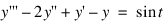
This example solves the third-order linear equation:
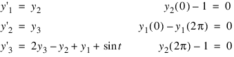
subject to the boundary conditions y(0) = y(2π) and y'(0) = y'(2π) = 1. (Its solution is y = sint.) To use the ODEBV function, the problem is reduced to a system of first-order equations by defining y1 = y, y2 = y' and y3 = y''. The resulting system is:
Note that one boundary condition is at the left endpoint t = 0 and one boundary condition coupling is at the left and right endpoints. The final boundary condition is at the right endpoint. The number of boundary conditions must be the same as the number of equations (in this case 3).
FUNCTION fcneqn0, x, y
RETURN, [ y(1), y(2), 2*y(2)-y(1)+y(0)+sin(x) ]
END
FUNCTION fcnjac0, x, y
RETURN, [ [0,1,0], [0,0,1], [1,-1,2] ]
END
FUNCTION fcnbc0, yleft, yright
RETURN, [ yleft(1)-1, yleft(0)-yright(0), yright(1)-1 ]
END
PRO odebvex0, y, e
MATH_INIT
y = ODEBV('fcneqn0','fcnjac0','fcnbc0',3,1,1,0, $ 2*3.1415927, /linear, err = e)
END
Example 2
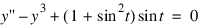
In this example, the following nonlinear problem is solved:
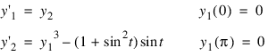
with y(0) = y(π) = 0. Its solution is y = sint. As in Example 1, this equation is reduced to a system of first-order differential equations by defining y1 = y and y2 = y'. The resulting system is:
In this problem, there is one boundary condition at the left endpoint and one at the right endpoint.
FUNCTION fcneqn1, x, y
RETURN, [ y(1), y(0)^3-sin(x)^3-sin(x) ]
END
FUNCTION fcnjac1, x, y
RETURN, [ [0,1], [3*y(0)*y(0),0] ]
END
FUNCTION fcnbc1, yleft, yright
RETURN, [ yleft(0), yright(0) ]
END
PRO odebvex1, y, e
MATH_INIT
i = INTERPOL( [0,!dpi], 12 )
i = [ [i], [0.4*i*(!dpi-i)], [0.4*(!dpi-2*i)] ]
y = ODEBV( 'fcneqn1', 'fcnjac1', 'fcnbc1', 2, 1, 0, 0, $
!dpi, init=i, err=e )
END
Example 3
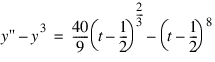
In this example, the following nonlinear problem is solved:
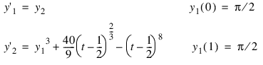
with y(0) = y(1) = π/2. As in the previous examples, this equation is reduced to a system of first-order differential equations by defining y1 = y and y2 = y'. The resulting system is:
FUNCTION fcneqn2, x, y
z = x - 0.5d
z = z * z
RETURN, [ y(1), $
y(0)^3+4.444444444444444d*z^(0.3333333333333333d)-z^4 ]
END
FUNCTION fcnjac2, x, y
RETURN, [ [0d,1d], [3d*y(0)*y(0),0d] ]
END
FUNCTION fcnbc2, yleft, yright
RETURN, [ yleft(0) - 1.570796326794896d, $
yright(0) - 1.570796326794896d ]
END
PRO odebvex2, y, e
MATH_INIT
i = [ [0.0,0.4,0.5,0.6,1.0], $
[0.15749,0.00215,0.0,0.00215,0.15749] ]
i = [ [i], [-0.83995,-0.05745,0.0,0.05745,0.83995] ]
y = ODEBV( 'fcneqn2', 'fcnjac2', 'fcnbc2', 2, 1, 0, 0, 1, $
init = i, err = e )
END
Version 2017.0
Copyright © 2017, Rogue Wave Software, Inc. All Rights Reserved.