KOLMOGOROV1 Function (PV-WAVE Advantage)
Performs a Kolmogorov-Smirnov one-sample test for continuous distributions.
Usage
result = KOLMOGOROV1(f, x)
Input Parameters
f—Scalar string specifying a user-supplied function to compute the cumulative distribution function (CDF) at a given value. Parameter f accepts the following parameter and returns the computed function value at this point:
 y
y—Point at which the function is to be evaluated.
x—One-dimensional array containing the observations.
Returned Value
result—One-dimensional array of length 3 containing Z, p1, and p2 .
Input Keywords
Double—If present and nonzero, double precision is used.
Output Keywords
Differences—Named variable into which an array containing Dn , Dn+, Dn- is stored.
Nmissing—Named variable into which the number of missing values is stored.
Discussion
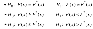
The function KOLMOGOROV1 performs a Kolmogorov-Smirnov goodness-of-fit test in one sample. The hypotheses tested follow:
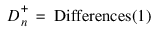
where F is the cumulative distribution function (CDF) of the random variable, and the theoretical CDF, F*, is specified via the user-supplied function f. Let n = N_ELEMENTS(x) − Nmissing. The test statistics for both one-sided alternatives:
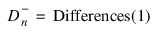
and:
and the two-sided (Dn = Differences(0)) alternative are computed as well as an asymptotic z-score (result(0)) and p-values associated with the one-sided (result(1)) and two-sided (result(2)) hypotheses. For n > 80, asymptotic p-values are used (see Gibbons 1971). For n ≤ 80, exact one-sided p-values are computed according to a method given by Conover (1980, page 350). An approximate two-sided test p-value is obtained as twice the one-sided p-value. The approximation is very close for one-sided p-values less than 0.10 and becomes very bad as the one-sided p-values get larger.
Programming Notes
1. The theoretical CDF is assumed to be continuous. If the CDF is not continuous, the statistics:
will not be computed correctly.
2. Estimation of parameters in the theoretical CDF from the sample data will tend to make the p-values associated with the test statistics too liberal. The empirical CDF will tend to be closer to the theoretical CDF than it should be.
3. No attempt is made to check that all points in the sample are in the support of the theoretical CDF. If all sample points are not in the support of the CDF, the null hypothesis must be rejected.
Example
In this example, a random sample of size 100 is generated via routine RANDOM for the uniform (0, 1) distribution. We want to test the null hypothesis that the CDF is the standard normal distribution with a mean of 0.5 and a variance equal to the uniform (0, 1) variance (1/12).
FUNCTION l_Cdf, x
mean = 0.5
std = 0.2886751
z = (x - mean)/std
val = NORMALCDF(z)
RETURN, val
END
RANDOMOPT, set = 123457
x = RANDOM(100, /Uniform)
stats = KOLMOGOROV1('l_cdf', x, Differences = d, Nmissing = nm)PRINT, 'D =', d(0)
; PV-WAVE prints: D = 0.147083
PRINT, 'D+ =', d(1)
; PV-WAVE prints: D+ = 0.0809559
PRINT, 'D- =', d(2)
; PV-WAVE prints: D- = 0.147083
PRINT, 'Z =', stats(0)
; PV-WAVE prints: Z = 1.47083
PRINT, 'Prob greater D one sided =', stats(1)
; PV-WAVE prints: Prob greater D one sided = 0.0132111
Version 2017.0
Copyright © 2017, Rogue Wave Software, Inc. All Rights Reserved.