QUADPROG Function (PV-WAVE Advantage)
Solves a quadratic programming (QP) problem subject to linear equality or inequality constraints.
Usage
result = QUADPROG(a, b, g, h)
Input Parameters
a—Two-dimensional matrix containing the linear constraints.
b—One-dimensional matrix of the right-hand sides of the linear constraints.
g—One-dimensional array of the coefficients of the linear term of the objective function.
h—Two-dimensional array of size N_ELEMENTS(g) × N_ELEMENTS(g) containing the Hessian matrix of the objective function. It must be symmetric positive definite. If h is not positive definite, the algorithm attempts to solve the QP problem with h replaced by h + diag*I, such that h + diag*I is positive definite.
Returned Value
result—The solution x of the QP problem.
Input Keywords
Double—If present and nonzero, double precision is used.
Meq—Number of linear equality constraints. If Meq is used, then the equality constraints are located at a(i, *) for i = 0, ..., Meq – 1. Default: Meq = N_ELEMENTS(a(*, 0)) n; i.e., all constraints are equality constraints
Output Keywords
Diag—Name of the variable into which the scalar, equal to the multiple of the identity matrix added to h to give a positive definite matrix, is stored.
Dual—Name of the variable into which an array with N_ELEMENTS(g) elements, containing the Lagrange multiplier estimates, is stored.
Obj—Name of variable into which optimal object function found is stored.
Discussion
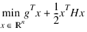
Function QUADPROG is based on M.J.D. Powell’s implementation of the Goldfarb and Idnani dual quadratic programming (QP) algorithm for convex QP problems subject to general linear equality/inequality constraints (Goldfarb and Idnani 1983). I.e., problems of the form:
subject to:
given the vectors b0, b1, and g, and the matrices H, A0, and A1. Matrix H is required to be positive definite. In this case, a unique x solves the problem, or the constraints are inconsistent. If H is not positive definite, a positive definite perturbation of H is used in place of H. For more details, see Powell (1983, 1985).
If a perturbation of H, H + αI, is used in the QP problem, H + αI also should be used in the definition of the Lagrange multipliers.
Example
The QP problem:
min f(x) = –x20 + x21 + x22 + x23 + x24 – 2x1x2 – 2x3x4 –2x0
subject to:
x0 + x1 + x2 + x3 + x4 = 5
x2 – 2x3 – 2x4 = –3
is solved.
; Define the coefficient matrix A.
a = transpose( $
[[1,1,1,1,1], $
[0,0,1,-2,-2]])
; Define the Hessian matrix of the objective function. Notice
; that since h is symmetric, the array concatenation operators
; "[ ]" are used to define it.
h = [[2, 0, 0, 0, 0], [0, 2, -2, 0, 0], $
[0, -2, 2, 0, 0], [0, 0, 0, 2, -2], $
[0, 0, 0, -2, 2]]
; Define b.
b = [5, -3]
; Define g.
g = [ -2, 0, 0, 0, 0]
; Call QUADPROG.
x = QUADPROG(a, b, g, h)
; Output solution.
PM, x
; This results in the following output:
; 1.00000
; 1.00000
; 1.00000
; 1.00000
; 1.00000
Warning Errors
MATH_NO_MORE_PROGRESS—Due to the effect of computer rounding error, a change in the variables fails to improve the objective function value. Usually, the solution is close to optimum.
Fatal Errors
MATH_SYSTEM_INCONSISTENT—System of equations is inconsistent. There is no solution.
Version 2017.0
Copyright © 2017, Rogue Wave Software, Inc. All Rights Reserved.