model—Four element array containing the numbers p, q, s, d of the ARIMA  model the outlier free series is following.
model the outlier free series is following. model the outlier free series is following. :
:
 ,
,  , and
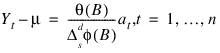
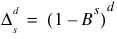
, and 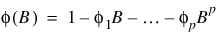 . B is the lag operator,
 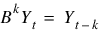 , {at} is a white noise process, and μ denotes the mean of the series {Yt}.
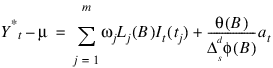
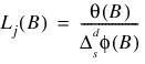
 is the observed outlier contaminated series, and ωj and Lj(B) denote the magnitude and dynamic pattern of outlier j, respectively. It(tj) is an indicator function that determines the temporal course of the outlier effect,
  , It(tj) = 0 otherwise.
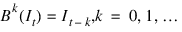
 by removing all occurring outlier effects:
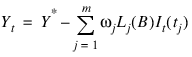
 for an innovational outlier
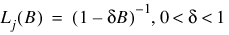 for a temporary change outlier
 series = [ 0.24300E01, 0.25060E01, 0.27670E01, 0.29400E01, $
0.31690E01, 0.34500E01, 0.35940E01, 0.37740E01, $
0.36950E01, 0.34110E01, 0.27180E01, 0.19910E01, $
0.22650E01, 0.24460E01, 0.26120E01, 0.33590E01, $
0.34290E01, 0.35330E01, 0.32610E01, 0.26120E01, $
0.21790E01, 0.16530E01, 0.18320E01, 0.23280E01, $
0.27370E01, 0.30140E01, 0.33280E01, 0.34040E01, $
0.29810E01, 0.25570E01, 0.25760E01, 0.23520E01, $
0.25560E01, 0.28640E01, 0.32140E01, 0.34350E01, $
0.34580E01, 0.33260E01, 0.28350E01, 0.24760E01, $
0.23730E01, 0.23890E01, 0.27420E01, 0.32100E01, $
0.35200E01, 0.38280E01, 0.36280E01, 0.28370E01, $
0.24060E01, 0.26750E01, 0.25540E01, 0.28940E01, $
0.32020E01, 0.32240E01, 0.33520E01, 0.31540E01, $
0.28780E01, 0.24760E01, 0.23030E01, 0.23600E01, $
0.26710E01, 0.28670E01, 0.33100E01, 0.34490E01, $
0.36460E01, 0.34000E01, 0.25900E01, 0.18630E01, $
0.15810E01, 0.16900E01, 0.17710E01, 0.22740E01, $
0.25760E01, 0.31110E01, 0.36050E01, 0.35430E01, $
0.27690E01, 0.20210E01, 0.21850E01, 0.25880E01, $
0.28800E01, 0.31150E01, 0.35400E01, 0.38450E01, $
0.38000E01, 0.35790E01, 0.32640E01, 0.25380E01, $
0.25820E01, 0.29070E01, 0.31420E01, 0.34330E01, $
0.35800E01, 0.34900E01, 0.34750E01, 0.35790E01, $
0.28290E01, 0.19090E01, 0.19030E01, 0.20330E01, $
0.23600E01, 0.26010E01, 0.30540E01, 0.33860E01, $
0.35530E01, 0.34680E01, 0.31870E01, 0.27230E01, $
0.26860E01, 0.28210E01, 0.30000E01, 0.32010E01, $
0.34240E01, 0.35310E01]
n_obs = N_ELEMENTS(series) ; 114
model = [2, 0, 1, 2]
result = TS_OUTLIER_IDENTIFICATION( $
model, series, Critical=3.5, $
Num_outliers=num_outliers, $
Outlier_statistics=outlier_stat, $
Arma_param=parameters, $
Res_sigma=res_sigma, $
Aic=aic)
PRINT, "ARMA parameters:"
p = model(0) + model(1)
PRINT, parameters(0:p), Format='(F11.6)'
PRINT, ''
PRINT, num_outliers, Format="('Number of outliers: ', I1)"PRINT, ''
PRINT, "Outlier statistics:"
PRINT, "Time point Outlier type"
FOR i=0L, num_outliers-1 DO $
PRINT, outlier_stat(2*i), outlier_stat(2*i+1), $
Format="(I6, 10X, I3)"
PRINT, ''
PRINT, res_sigma, Format="('RSE: ', F10.6)"PRINT, aic, Format="('AIC: ', F10.6)"PRINT, ''
; Print out the first 36 values of result and series
PRINT, "Extract from the series:"
PRINT, ''
PRINT, "Time point Original Series Outlier free series"
FOR i=0L, 35 DO $
PRINT, (i+1), series(i), result(i), $
Format='(I6, F17.6, F18.6)'
ARMA parameters:
0.000000
0.106532
-0.195856
Number of outliers: 1
Outlier statistics:
Time point Outlier type
16 2
RSE: 0.319542
AIC: 282.918152
Extract from the series:
Time point Original Series Outlier free series
1 2.430000 2.430000
2 2.506000 2.506000
3 2.767000 2.767000
4 2.940000 2.940000
5 3.169000 3.169000
6 3.450000 3.450000
7 3.594000 3.594000
8 3.774000 3.774000
9 3.695000 3.695000
10 3.411000 3.411000
11 2.718000 2.718000
12 1.991000 1.991000
13 2.265000 2.265000
14 2.446000 2.446000
15 2.612000 2.612000
16 3.359000 2.699728
17 3.429000 2.769728
18 3.533000 2.873728
19 3.261000 2.601728
20 2.612000 1.952728
21 2.179000 1.519728
22 1.653000 0.993728
23 1.832000 1.172728
24 2.328000 1.668728
25 2.737000 2.077728
26 3.014000 2.354728
27 3.328000 2.668728
28 3.404000 2.744728
29 2.981000 2.321728
30 2.557000 1.897728
31 2.576000 1.916728
32 2.352000 1.692728
33 2.556000 1.896728
34 2.864000 2.204728
35 3.214000 2.554728
36 3.435000 2.775728
n_obs = 300
series = [ 50.0000000, 50.2728081, 50.6242599, 51.0373917, $
51.9317627, 50.3494759, 51.6597252, 52.7004929, $
53.5499802, 53.1673279, 50.2373505, 49.3373871, $
49.5516472, 48.6692696, 47.6606636, 46.8774185, $
45.7315445, 45.6469727, 45.9882355, 45.5216560, $
46.0479660, 48.1958656, 48.6387749, 49.9055367, $
49.8077278, 47.7858467, 47.9386749, 49.7691956, $
48.5425873, 49.1239853, 49.8518791, 50.3320694, $
50.9146347, 51.8772049, 51.8745689, 52.3394470, $
52.7273712, 51.4310036, 50.6727448, 50.8370399, $
51.2843437, 51.8162918, 51.6933670, 49.7038231, $
49.0189247, 49.455703 , 50.2718010, 49.9605980, $
51.3775749, 50.2285385, 48.2692299, 47.6495590, $
49.2938499, 49.1924858, 49.6449242, 50.0446815, $
51.9972496, 54.2576981, 52.9835434, 50.4193535, $
50.3617897, 51.8276901, 53.1239929, 54.0682144, $
54.9238319, 55.6877632, 54.8896332, 54.0701065, $
52.2754097, 52.2522354, 53.1248703, 51.1287193, $
50.5003815, 49.6504173, 47.2453079, 45.4555626, $
45.8449707, 45.9765129, 45.7682228, 45.2343674, $
46.6496811, 47.0894432, 49.3368340, 50.8058052, $
49.9132500, 49.5893288, 48.2470627, 46.9779968, $
45.6760864, 45.7070389, 46.6158409, 47.5303612, $
47.5630417, 47.0389214, 46.0352287, 45.8161545, $
45.7974396, 46.0015373, 45.3796463, 45.3461685, $
47.6444016, 49.3327446, 49.3810692, 50.2027817, $
51.4567032, 52.3986320, 52.5819206, 52.7721825, $
52.6919098, 53.3274345, 55.1345940, 56.8962631, $
55.7791634, 55.0616989, 52.3551178, 51.3264084, $
51.0968323, 51.1980476, 52.8001442, 52.0545082, $
50.8742943, 51.5150337, 51.2242050, 50.5033989, $
48.7760124, 47.4179192, 49.7319527, 51.3320541, $
52.3918304, 52.4140434, 51.0845947, 49.6485748, $
50.6893463, 52.9840813, 53.3246994, 52.4568024, $
51.9196091, 53.6683121, 53.4555359, 51.7755814, $
49.2915611, 49.8755112, 49.4546776, 48.6171913, $
49.9643021, 49.3766441, 49.2551308, 50.1021881, $
51.0769119, 55.8328133, 52.0212708, 53.4930801, $
53.2147255, 52.2356453, 51.9648819, 52.1816330, $
51.9898071, 52.5623627, 51.0717278, 52.2431946, $
53.6943054, 54.3752098, 54.1492615, 53.8523254, $
52.1093712, 52.3982697, 51.2405128, 50.3018112, $
51.3819618, 49.5479546, 47.5024452, 47.4447708, $
47.8939056, 48.4070015, 48.2440681, 48.7389755, $
49.7309227, 49.1998024, 49.5798340, 51.1196213, $
50.6288414, 50.3971405, 51.6084099, 52.4564743, $
51.6443901, 52.4080658, 52.4643364, 52.6257210, $
53.1604691, 51.9309731, 51.4137230, 52.1233368, $
52.9867249, 53.3180733, 51.9647636, 50.7947655, $
52.3815842, 50.8353729, 49.4136009, 52.8355217, $
52.2234840, 51.1392517, 48.5245132, 46.8700218, $
46.1607285, 45.2324257, 47.4157829, 48.9989090, $
49.6230736, 50.4352913, 51.1652985, 50.2588654, $
50.7820129, 51.0448799, 51.2880516, 49.6898804, $
49.0288200, 49.9338837, 48.2214432, 46.2103348, $
46.9550171, 47.5595894, 47.7176018, 48.4502945, $
50.9816895, 51.6950073, 51.6973495, 52.1941261, $
51.8988075, 52.5617599, 52.0218391, 49.5236053, $
47.9684906, 48.2445183, 48.8275146, 49.7176971, $
51.5649338, 52.5627213, 52.0182419, 50.9688835, $
51.5846901, 50.9486771, 48.8685837, 48.5600624, $
48.4760094, 48.5348396, 50.4187813, 51.2542381, $
50.1872864, 50.4407692, 50.6222687, 50.4972000, $
51.0036087, 51.3367500, 51.7368202, 53.0463791, $
53.6261253, 52.0728683, 48.9740753, 49.3280830, $
49.2733917, 49.8519020, 50.8562126, 49.5594254, $
49.6109200, 48.3785629, 48.0026474, 49.4874268, $
50.1596375, 51.8059540, 53.0288620, 51.3321075, $
49.3114815, 48.7999306, 47.7201881, 46.3433914, $
46.5303612, 47.6294632, 48.6012459, 47.8567657, $
48.0604057, 47.1352806, 49.5724792, 50.5566483, $
49.4182968, 50.5578079, 50.6883736, 50.6333389, $
51.9766159, 51.0595245, 49.3751640, 46.9667702, $
47.1658173, 47.4411278, 47.5360374, 48.9914742, $
50.4747620, 50.2728043, 51.9117165, 53.7627792]
model = [1, 1, 1, 0]
result = TS_OUTLIER_IDENTIFICATION( $
model, series, $
Num_outliers=num_outliers, $
Outlier_statistics=outlier_stat, $
Omega_weights=omega_user, $
Arma_param=parameters_user, $
Res_sigma=res_sigma, $
Aic=aic, $
Relative_Error=1.0e-5)
PRINT, "ARMA parameters:"
p = N_ELEMENTS(parameters_user)
PRINT, parameters_user(0:(p-1)), Format='(F11.6)'
PRINT, ''
PRINT, num_outliers, Format="('Number of outliers: ', I1)"PRINT, ''
PRINT, "Outlier statistics:"
PRINT, "Time point Outlier type"
FOR i=0L, num_outliers-1 DO $
PRINT, outlier_stat(i,0), outlier_stat(i,1), $
Format="(I6, 10X, I3)"
PRINT, ''
PRINT, "Omega statistics:"
PRINT, "Time point Omega"
FOR i=0L, num_outliers-1 DO $
PRINT, outlier_stat(i,0), omega_user(i), $
Format="(I6, 6X, F11.6)"
PRINT, ''
PRINT, res_sigma, Format="('RSE: ', F11.6)"PRINT, aic, Format="('AIC: ', F11.6)"ARMA parameters:
10.828934
0.785221
-0.496502
Number of outliers: 2
Outlier statistics:
Time point Outlier type
150 1
200 3
Omega statistics:
Time point Omega
150 4.477869
200 3.381565
RSE: 1.007222
AIC: 1417.044067