CROSSCORRELATION Function (PV-WAVE Advantage)
Computes the sample cross-correlation function of two stationary time series.
Usage
result = CROSSCORRELATION (x, y, lagmax)
Input Parameters
x—Array of length n_observations containing the first time series, where n_observations is the number of observations in each time series.
y—Array of length n_observations containing the second time series.
lagmax—Maximum lag of cross-covariances and cross-correlations to be computed. lagmax must be greater than or equal to 1 and less than n_observations.
Returned Value
result—Array of length 2 * lagmax + 1 containing the cross-correlations between the time series x and y. The kth element of this array contains the cross-correlation between x and y at lag (k-lagmax) where k = 0, 1, …, 2 * lagmax.
Input Keywords
Double—If present and nonzero, double precision is used.
Input_means—A 2 element array containing the user input of the estimate of the mean of the time series x at Input_means(0) and the user input of the estimate of the mean of the time series y at Input_means(1).
Std_error_option—An integer used to select the method of compilation for standard errors of the cross-correlations.

1—Compute standard errors of cross-correlations using Bartlett’s formula.
2—Compute standard errors of cross-correlations using Bartlett’s formula with the assumption of no cross-correlation.
Output Keywords
Variances—A 2 element array containing the variance of the time series x at Variances(0) and variance of the time series y at Variances(1).
Std_errors—Array of length 2 * lagmax + 1 containing the standard errors of the cross-correlations between the time series x and y. Method of computation for standard errors of the cross-correlations is chosen by the Std_error_options keyword.
Cross_covariances—Array of length 2 * lagmax + 1 containing the cross-covariances between the time series x and y. The kth element of this array contains the cross-covariances between x and y at lag (k–lagmax) where k = 0, 1, …, 2 * lagmax.
Output_means—A 2 element array containing the mean of the time series x at Output_means(0) and the mean of the time series y at Output_means(1).
Discussion
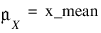
CROSSCORRELATION estimates the cross-correlation function of two jointly stationary time series given a sample of n = n_observations observations {Xt} and {Yt} for t = 1, 2, …, n. Let:
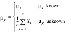
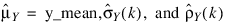
be the estimate of the mean μX of the time series {Xt} where:
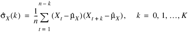
The autocovariance function of {Xt}, σX(k), is estimated by:
where K = lagmax. Note that:
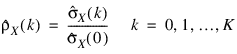
is equivalent to the sample variance x_variance. The autocorrelation function ρX(k) is estimated by:
Note that:
by definition. Let:
be similarly defined.
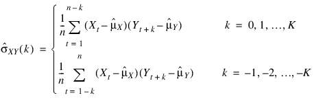
The cross-covariance function σXY(k) is estimated by:
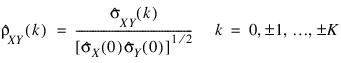
The cross-correlation function ρXY(k) is estimated by:
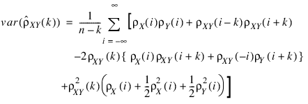
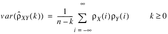
The standard errors of the sample cross-correlations may be optionally computed according to the Std_error_options option for the Std_errors keyword. One method is based on a general asymptotic expression for the variance of the sample cross-correlation coefficient of two jointly stationary time series with independent, identically distributed normal errors given by Bartlett (1978, page 352). The theoretical formula is:
For computational purposes, the autocorrelations ρX(k) and ρY(k) and the cross-correlations ρXY(k) are replaced by their corresponding estimates for |k| ≤ K, and the limits of summation are equal to zero for all k such that |k| > K.
A second method evaluates Bartlett’s formula under the additional assumption that the two series have no cross-correlation. The theoretical formula is:
For additional special cases of Bartlett’s formula, see Box and Jenkins (1976, page 377).
An important property of the cross-covariance coefficient is σXY(k) = σYX(–k) for k ≥ 0. This result is used in the computation of the standard error of the sample cross-correlation for lag k < 0. In general, the cross-covariance function is not symmetric about zero so both positive and negative lags are of interest.
Example
Consider the Gas Furnace Data (Box and Jenkins 1976, pages 532–533) where X is the input gas rate in cubic feet/minute and Y is the percent CO2 in the outlet gas. CROSSCORRELATION is used to compute the cross-covariances and cross-correlations between time series X and Y with lags from –lagmax = –10 through lag lagmax = 10. In addition, the estimated standard errors of the estimated crosscorrelations are computed. The standard errors are based on the additional assumption that all cross-correlations for X and Y are zero.
; Retrieve and set up the Gas Furnace Data
data = STATDATA(7)
nobs = 296
lagmax = 10
x = FLTARR(nobs)
y = FLTARR(nobs)
x = data(*,0)
y = data(*,1)
cc = CROSSCORRELATION(x, y, lagmax, $
Output_means=output_means, $
Variances=variances, $
Std_error_option=2, $
Std_errors=std_errors, $
Cross_covariances=cross_covariances)
;
; Display the output
print,""
PRINT," OUTPUT"
print,"================"
print,""
PRINT,"Mean of series X = ", output_means(0)
PRINT,"Variance of series X = ", variances(0)
PRINT,""
PRINT,"Mean of series Y = ", output_means(1)
PRINT,"Variance of series Y = ", variances(1)
PRINT,""
PRINT," Lag CROSS_COV CC STD_ERRORS"
PRINT," --- --------- ---- ----------"
FOR i=0L, 2*lagmax DO $
PRINT,i - lagmax, cross_covariances(i), cc(i), std_errors(i)
Output
OUTPUT
================
Mean of series X = -0.0568344
Variance of series X = 1.14694
Mean of series Y = 53.5091
Variance of series Y = 10.2189
Lag CROSS_COV CC STD_ERRORS
--- --------- ---- ----------
-10 -0.404502 -0.118154 0.162754
-9 -0.508491 -0.148529 0.162470
-8 -0.614369 -0.179456 0.162188
-7 -0.705476 -0.206067 0.161907
-6 -0.776167 -0.226716 0.161627
-5 -0.831474 -0.242871 0.161349
-4 -0.891316 -0.260351 0.161073
-3 -0.980605 -0.286432 0.160798
-2 -1.12477 -0.328542 0.160524
-1 -1.34704 -0.393467 0.160252
0 -1.65853 -0.484451 0.159981
1 -2.04865 -0.598405 0.160252
2 -2.48217 -0.725033 0.160524
3 -2.88541 -0.842820 0.160798
4 -3.16536 -0.924592 0.161073
5 -3.25344 -0.950319 0.161349
6 -3.13113 -0.914593 0.161627
7 -2.83919 -0.829320 0.161907
8 -2.45302 -0.716521 0.162188
9 -2.05269 -0.599584 0.162470
10 -1.69466 -0.495004 0.162754
Version 2017.0
Copyright © 2017, Rogue Wave Software, Inc. All Rights Reserved.