PARTIAL_AC Function (PV-WAVE Advantage)
Computes the sample partial autocorrelation function of a stationary time series.
Usage
result = PARTIAL_AC(cf)
Input Parameters
cf—One-dimensional array containing the autocorrelations of the time series x.
Returned Value
result—One-dimensional array containing the partial autocorrelations of the time series x.
Input Keywords
Double—If present and nonzero, double precision is used.
Discussion
PARTIAL_AC estimates the partial autocorrelations of a stationary time series given the K = (N_ELEMENTS(cf) – 1) sample autocorrelations:
for k = 0, 1, ..., K. Consider the AR(k) process defined by:
where φkj denotes the jth coefficient in the process. The set of estimates:
for k = 1, ..., K is the sample partial autocorrelation function. The autoregressive parameters:
for j = 1, ..., k are approximated by Yule-Walker estimates for successive AR(k) models where k = 1, ..., K. Based on the sample Yule-Walker equations:
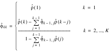
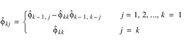
a recursive relationship for k = 1, ..., K was developed by Durbin (1960). The equations are given by:
and:
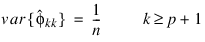
This procedure is sensitive to rounding error and should not be used if the parameters are near the nonstationarity boundary. A possible alternative would be to estimate {φkk} for successive AR(k) models using least or maximum likelihood. Based on the hypothesis that the true process is AR(p), Box and Jenkins (1976, page 65) note:
See Box and Jenkins (1976, pages 82–84) for more information concerning the partial autocorrelation function.
Example
Consider the Wolfer Sunspot Data (Anderson 1971, page 660) consisting of the number of sunspots observed each year from 1749 through 1924. The data set for this example consists of the number of sunspots observed from 1770 through 1869. Routine PARTIAL_AC is used to compute the estimated partial autocorrelations.
data = STATDATA(2)
x = data(21:120,1)
result = AUTOCORRELATION(x, 20)
partial = PARTIAL_AC(result)
PRINT, 'LAG PACF'
FOR i=0L, 19 DO PM, i + 1, partial(i), Format = '(I2, F11.3)'
This results in the following output:
LAG PACF
1 0.806
2 -0.635
3 0.078
4 -0.059
5 -0.001
6 0.172
7 0.109
8 0.110
9 0.079
10 0.079
11 0.069
12 -0.038
13 0.081
14 0.033
15 -0.035
16 -0.131
17 -0.155
18 -0.119
19 -0.016
20 -0.004
Version 2017.0
Copyright © 2017, Rogue Wave Software, Inc. All Rights Reserved.