ESTIMATE_MISSING Function (PV-WAVE Advantage)
Estimates missing values in a time series.
Usage
result = ESTIMATE_MISSING(tpoints, z)
Input Parameters
tpoints—Array of length n_obs containing the time points t1, ..., tn_obs at which the time series values were observed. n_obs is the number of non-missing observations in the time series. The time points must be in strictly increasing order. Time points for missing values must lie in the open interval (t1, tn_obs).
z—Array of length n_obs containing the time series values. The values must be ordered in accordance with the values in array tpoints. It is assumed that the time series after estimation of missing values contains values at equidistant time points where the distance between two consecutive time points is one. If the non-missing time series values are observed at time points t1, ..., tn_obs, then missing values between ti and ti+1, i = 1, ..., n_obs – 1, exist if ti+1 – ti > 1. The size of the gap between ti and ti+1 is then ti+1 – ti – 1. The total length of the time series with non-missing and estimated missing values is tn_obs – ti + 1, or tpoints(n_obs – 1) – tpoints(0) + 1.
Returned Value
result—Array of length (tpoints(n_obs – 1) – tpoints(0) + 1) containing the time series together with estimates for the missing values.
Input Keywords
Double—If present and nonzero, double precision is used.
Method—The method used for estimating the missing values:

0—Use median.
1—Use cubic spline interpolation.
2—Use one-step-ahead forecasts from an AR(1) model.
3—Use one-step-ahead forecasts from an AR(p) model. This is the default.
If
Method = 2 is chosen, then all values of gaps beginning at time points
t1 + 1
or
t1 + 2 are estimated by
Method 0. If
Method = 3 is chosen and the first gap starts at
t1 + 1, then the values of this gap are also estimated by
Method 0. If the length of the series before a gap, denoted
len, is greater than 1 and less than

, then maxlag is reduced to
len/2 for the computation of the missing values within this gap. Default
Method = 3.
Maxlag—A scalar value indicating the maximum lag number when Method = 3 was chosen. Default: Maxlag = 10
Mean_estimate—Estimate of the mean of the time series.
Convergence_tolerance—Tolerance level used to determine convergence of the nonlinear least squares algorithm used if Method = 2. Convergence_tolerance represents the minimum relative decrease in the sum of squares between two iterations required to determine convergence. Hence, Convergence_tolerance must be greater than or equal to 0.
Relative_error—Stopping criterion for use in the nonlinear equation solver used if Method = 2.
Maxit—A scalar value indicating the maximum number of iterations allowed in the nonlinear equations solver used if Method = 2. Default: Maxit = 200.
Output Keywords
Ntimes—Number of elements in the time series with estimated missing values. Note that Ntimes = tpoints(n_obs – 1) – tpoints(0) + 1.
Times_array—Array of length Ntimes = tpoints(n_obs – 1) – tpoints(0) + 1 containing the time points of the time series with estimates for the missing values.
Missing_index—Array of length (Ntimes – n_obs) containing the indices for the missing values in Times_array. If Ntimes – n_obs = 0, then this keyword is not valid.
Discussion
Traditional time series analysis as described by Box, Jenkins and Reinsel (1994) requires the observations made at equidistant time points t1, t1 + 1, t1 + 2, ..., tn. When observations are missing, the problem occurs to determine suitable estimates. ESTIMATE_MISSING offers 4 estimation methods:
Method 0 estimates the missing observations in a gap by the median of the last four time series values before and the first four values after the gap. If not enough values are available before or after the gap then the number is reduced accordingly. This method is very fast and simple, but its use is limited to stationary ergodic series without outliers and level shifts.
Method 1 uses a cubic spline interpolation method to estimate missing values. Here the interpolation is again done over the last four time series values before and the first four values after the gap. The missing values are estimated by the resulting interpolant. This method gives smooth transitions across missing values.
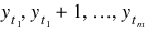
Method 2 assumes that the time series before the gap can be well described by an AR(1) process. If the last observation prior to the gap is made at time point
tm then it uses the time series values at
t1,
t1 + 1, ...,
tm to compute the one-step-ahead forecast at origin
tm. This value is taken as an estimate for the missing value at time point
tm + 1. If the value at
tm + 2 is also missing then the values at time points
t1,
t1 + 1, ...,
tm + 1 are used to recompute the AR(1) model, estimate the value at
tm + 2 and so on. The coefficient
φ1 in the AR(1) model is computed internally by the method of least squares from ARMA.
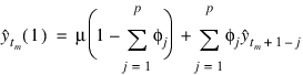
Finally, method 3 uses an AR(p) model to estimate missing values by a one-step-ahead forecast. First, AUTO_UNI_AR, applied to the time series prior to the missing values, is used to determine the optimum
p from the set {0, 1, ...,
Maxlag} of possible values and to compute the parameters
φ1, ...,
φp of the resulting AR(p) model. The parameters are estimated by the least squares method based on Householder transformations as described in Kitagawa and Akaike (1978). Denoting the mean of the series
by
μ the one-step-ahead forecast at origin

, can be computed by the formula:
This value is used as an estimate for the missing value. The procedure starting with AUTO_UNI_AR is then repeated for every further missing value in the gap.
note | All four estimation methods treat gaps of missing values in increasing time order. |
Example
Consider the AR(1) process:
Yt = φ1Yt–1 + at, t = 1, 2, 3, ...
We assume that {
at} is a Gaussian white noise process,
. Then,
E[
Yt] = 0 and
VAR[
Yt] =
σ2/(1 –
φ12) (see Anderson, p. 174).
The time series in the code below was artificially generated from an AR(1) process characterized by φ1 = –0.7 and σ2 = 1 – φ12 = 0.51. This process is stationary with VAR[Yt] = 1. As initial value, Yt := a0 was taken. The sequence {at} was generated by a random number generator.
From the original series, we remove the observations at time points t=130, t=140, t=141, t=160, t=175, t=176. Then, ESTIMATE_MISSING is used to compute estimates for the missing values by all 4 estimation methods available. The estimated values are compared with the actual values.
maxlag = 20
times_1 = LONARR(200)
times_2 = LONARR(200)
x_1 = FLTARR(200)
x_2 = FLTARR(200)
y = [ 1.30540, -1.37166, 1.47905, -0.91059, 1.36191, $
-2.16966, 3.11254, -1.99536, 2.29740, -1.82474, $
-0.25445, 0.33519, -0.25480, -0.50574, -0.21429, $
-0.45932, -0.63813, 0.25646, -0.46243, -0.44104, $
0.42733, 0.61102, -0.82417, 1.48537, -1.57733, $
-0.09846, 0.46311, 0.49156, -1.66090, 2.02808, $
-1.45768, 1.36115, -0.65973, 1.13332, -0.86285, $
1.23848, -0.57301, -0.28210, 0.20195, 0.06981, $
0.28454, 0.19745, -0.16490, -1.05019, 0.78652, $
-0.40447, 0.71514, -0.90003, 1.83604, -2.51205, $
1.00526, -1.01683, 1.70691, -1.86564, 1.84912, $
-1.33120, 2.35105, -0.45579, -0.57773, -0.55226, $
0.88371, 0.23138, 0.59984, 0.31971, 0.59849, $
0.41873, -0.46955, 0.53003, -1.17203, 1.52937, $
-0.48017, -0.93830, 1.00651, -1.41493, -0.42188, $
-0.67010, 0.58079, -0.96193, 0.22763, -0.92214, $
1.35697, -1.47008, 2.47841, -1.50522, 0.41650, $
-0.21669, -0.90297, 0.00274, -1.04863, 0.66192, $
-0.39143, 0.40779, -0.68174, -0.04700, -0.84469, $
0.30735, -0.68412, 0.25888, -1.08642, 0.52928, $
0.72168, -0.18199, -0.09499, 0.67610, 0.14636, $
0.46846, -0.13989, 0.50856, -0.22268, 0.92756, $
0.73069, 0.78998, -1.01650, 1.25637, -2.36179, $
1.99616, -1.54326, 1.38220, 0.19674, -0.85241, $
0.40463, 0.39523, -0.60721, 0.25041, -1.24967, $
0.26727, 1.40042, -0.66963, 1.26049, -0.92074, $
0.05909, -0.61926, 1.41550, 0.25537, -0.13240, $
-0.07543, 0.10413, 1.42445, -1.37379, 0.44382, $
-1.57210, 2.04702, -2.22450, 1.27698, 0.01073, $
-0.88459, 0.88194, -0.25019, 0.70224, -0.41855, $
0.93850, 0.36007, -0.46043, 0.18645, 0.06337, $
0.29414, -0.20054, 0.83078, -1.62530, 2.64925, $
-1.25355, 1.59094, -1.00684, 1.03196, -1.58045, $
2.04295, -2.38264, 1.65095, -0.33273, -1.29092, $
0.14020, -0.11434, 0.04392, 0.05293, -0.42277, $
0.59143, -0.03347, -0.58457, 0.87030, 0.19985, $
-0.73500, 0.73640, 0.29531, 0.22325, -0.60035, $
1.42253, -1.11278, 1.30468, -0.41923, -0.38019, $
0.50937, 0.23051, 0.46496, 0.02459, -0.68478, $
0.25821, 1.17655, -2.26629, 1.41173, -0.68331]
tpoints = INDGEN(200) + 1
n_miss = 0
times_1(0) = tpoints(0)
times_2(0) = tpoints(0)
x_1(0) = y(0)
x_2(0) = y(0)
k = 0
FOR i=1L, N_ELEMENTS(tpoints)-1 DO BEGIN & $
times_1(i) = tpoints(i) & $
x_1(i) = y(i) & $
; Generate series with missing values
IF ((i NE 129) AND (i NE 139) AND (i NE 140) AND $
(i NE 159) AND (i NE 174) AND (i NE 175)) THEN BEGIN & $
k = k + 1 & $
times_2(k) = times_1(i) & $
x_2(k) = x_1(i) & $
ENDIF & $
ENDFOR
n_obs = k+1
times_tmp = times_2(0:n_obs-1)
x_tmp = x_2(0:n_obs-1)
FOR j=0L, 3 DO BEGIN & $
PRINT, "---- value of j is ", j & $
result = 0 & $
times = 0 & $
missing_index = 0 & $
IF (j LE 2) THEN BEGIN & $
result = ESTIMATE_MISSING( $
times_tmp, x_tmp, $
Method=j, $
Ntimes=ntimes, $
Times_Array=times, $
Missing_Index=missing_index) & $
ENDIF ELSE BEGIN & $
result = ESTIMATE_MISSING( $
times_tmp, x_tmp, $
Method=j, $
Ntimes=ntimes, $
Maxlag=maxlag, $
Times_Array=times, $
Missing_Index=missing_index) & $
ENDELSE & $
IF j EQ 0 THEN PRINT, "Method: Median" & $
IF j EQ 1 THEN PRINT, $
"Method: Cubic Spline Interpolation" & $
IF j EQ 2 THEN PRINT, "Method: AR(l) Forecast" & $
IF j EQ 3 THEN PRINT, "Method: AR(p) Forecast" & $
PRINT, ntimes, Format='("ntimes = ", I3)' & $ PRINT, $
"Time Actual Predicted Difference" & $
n_miss = ntimes - n_obs & $
FOR i=0L, n_miss-1 DO BEGIN & $
miss_ind = missing_index(i) & $
PRINT, times(miss_ind), x_1(miss_ind), $
result(miss_ind), ABS(x_1(miss_ind) - $
result(miss_ind)), $
Format='(I3, ",", F13.5, ",", F13.5, ",", F13.5)' & $
ENDFOR & $
PRINT, '' & $
ENDFOR
Output
Method: Median
ntimes = 200
Time Actual Predicted Difference
130, -0.92074, 0.26132, 1.18206
140, 0.44382, 0.05743, 0.38639
141, -1.57210, 0.05743, 1.62953
160, 2.64925, 0.04680, 2.60245
175, -0.42277, 0.04843, 0.47119
176, 0.59143, 0.04843, 0.54300
Method: Cubic Spline Interpolation
ntimes = 200
Time Actual Predicted Difference
130, -0.92074, 1.54109, 2.46183
140, 0.44382, -0.40730, 0.85112
141, -1.57210, 2.49709, 4.06919
160, 2.64925, -2.94712, 5.59637
175, -0.42277, 0.25066, 0.67343
176, 0.59143, 0.38032, 0.21111
Method: AR(l) Forecast
ntimes = 200
Time Actual Predicted Difference
130, -0.92074, -0.92971, 0.00897
140, 0.44382, 1.02824, 0.58442
141, -1.57210, -0.74527, 0.82683
160, 2.64925, 1.22880, 1.42045
175, -0.42277, 0.01049, 0.43326
176, 0.59143, 0.03683, 0.55460
Method: AR(p) Forecast
ntimes = 200
Time Actual Predicted Difference
130, -0.92074, -0.86385, 0.05689
140, 0.44382, 0.98098, 0.53716
141, -1.57210, -0.64489, 0.92721
160, 2.64925, 1.18966, 1.45959
175, -0.42277, -0.00105, 0.42172
176, 0.59143, 0.03773, 0.55370
Version 2017.0
Copyright © 2017, Rogue Wave Software, Inc. All Rights Reserved.