KALMAN Procedure (PV-WAVE Advantage)
Performs Kalman filtering and evaluates the likelihood function for the state-space model.
Usage
KALMAN, b, covb, n, ss, alndet
Input/Output Parameters
b—One dimensional array of containing the estimated state vector. The input is the estimated state vector at time k given the observations through time k – 1. The output is the estimated state vector at time k + 1 given the observations through time k. On the first call to KALMAN, the input b must be the prior mean of the state vector at time.
covb—Two dimensional array of size N_ELEMENTS(b) by N_ELEMENTS(b) such that covb* σ2 is the mean squared error matrix for b. Before the first call to KALMAN, covb* σ2 must equal the variance-covariance matrix of the state vector.
n—Named variable containing the rank of the variance-covariance matrix for all the observations. n must be initialized to zero before the first call to KALMAN. In the usual case when the variance-covariance matrix is nonsingular, n equals the sum of the N_ELEMENTS(Y) from the invocations to KALMAN. See the keyword section below for the definition of Y.
ss—Named vaiable containing the generalized sum of squares. ss must be initialized to zero before the first call to KALMAN. The estimate of σ2 is given by:
alndet—Named vaiable containing the natural log of the product of the nonzero eigenvalues of P where P * σ2 is the variance-covariance matrix of the observations. Although alndet is computed, KALMAN avoids the explicit computation of P. alndet must be initialized to zero before the first call to KALMAN. In the usual case when P is nonsingular, alndet is the natural log of the determinant of P.
Input Keywords
Y—One dimensional array containing the observations. Keywords Y, Z and R indicate an update step and must be used together
R—Two dimensional array if size N_ELEMENTS(Y) by N_ELEMENTS(Y) containing the matrix such that R * σ2 is the variance-covariance matrix of errors in the observation equation. Keywords Y, Z and R indicate an update step and must be used together.
T_matrix—Two dimensional array if size N_ELEMENTS(b) by N_ELEMENTS(b) containing the transition matrix in the state equation. Default: T_matrix = identity matrix
Q_matrix—Two dimensional array if size N_ELEMENTS(b) by N_ELEMENTS(b) matrix such that Q_matrix * σ2 is the variance-covariance matrix of the error vector in the state equation. Default: There is no error term in the state equation
Tolerance—Tolerance used in determining linear dependence. Default: Tolerance = 100*eps where eps is machine precision.
Output Keywords
V—One dimensional array of length N_ELEMENTS(Y) containing the one-step-ahead prediction error.
Covv—Two dimensional array if size N_ELEMENTS(Y) by N_ELEMENTS(Y) containing a matrix such that Covv * σ2 is the variance-covariance matrix of v.
Discussion
Routine KALMAN is based on a recursive algorithm given by Kalman (1960), which has come to be known as the Kalman filter. The underlying model is known as the state-space model. The model is specified stage by stage where the stages generally correspond to time points at which the observations become available. The routine KALMAN avoids many of the computations and storage requirements that would be necessary if one were to process all the data at the end of each stage in order to estimate the state vector. This is accomplished by using previous computations and retaining in storage only those items essential for processing of future observations.
The notation used here follows that of Sallas and Harville (1981). Let yk (input in keyword Y) be the nk × 1 vector of observations that become available at time k. The subscript k is used here rather than t, which is more customary in time series, to emphasize that the model is expressed in stages k = 1, 2, ... and that these stages need not correspond to equally spaced time points. In fact, they need not correspond to time points of any kind. The observation equation for the state-space model is:
yk = Zkbk + ek k = 1, 2, ...
Here, Zk is an nk × q known matrix and bk is the q × 1 state vector. The state vector bk is allowed to change with time in accordance with the state equation:
bk+1 = Tk+1 bk + wk+1 k = 1, 2, ...
starting with b1 = μ1 + w1.
The change in the state vector from time k to k + 1 is explained in part by the transition matrix Tk+1 (the identity matrix by default, or optionally input using keyword T_matrix), which is assumed known. It is assumed that the q-dimensional wks (k = 1, 2, ... K) are independently distributed multivariate normal with mean vector 0 and variance-covariance matrix σ2Qk, that the nk-dimensional eks (k = 1, 2, ... K) are independently distributed multivariate normal with mean vector 0 and variance-covariance matrix σ2Rk, and that the wks and eks are independent of each other. Here, μ1 is the mean of b1 and is assumed known, σ2 is an unknown positive scalar. Qk+1 (input in Q) and Rk (input in keyword R) are assumed known.
Denote the estimator of the realization of the state vector bk given the observations y1, y2, …, yj by:
By definition, the mean squared error matrix for:
is:
At the time of the kth invocation, we have:
and:
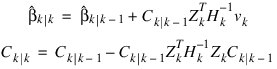
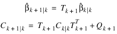
which were computed from the (k–1)st invocation, input in b and covb, respectively. During the kth invocation, routine KALMAN computes the filtered estimate:
along with Ck|k. These quantities are given by the update equations:
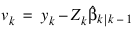
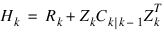
where:
and where:
Here, vk (stored in v) is the one-step-ahead prediction error, and σ2Hk is the variance-covariance matrix for vk. Hk is stored in covv. The “start-up values” needed on the first invocation of KALMAN are:
and C1|0 = Q1 input via b and covb, respectively. Computations for the kth invocation are completed by KALMAN computing the one-step-ahead estimate:
along with Ck+1|k given by the prediction equations:
If both the filtered estimates and one-step-ahead estimates are needed by the user at each time point, KALMAN can be invoked twice for each time point—first without T_matrix and Q_matrix to produce:
and Ck|k, and second without keywords Y, Z, and R to produce:
and Ck+1|k. Without T_matrix and Q_matrix, prediction equations are skipped. Without keywords Y, Z, and R, update equations are skipped.
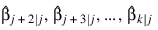
Often, one desires the estimate of the state vector more than one-step-ahead, i.e., an estimate of:
is needed where k > j + 1. At time j, KALMAN is invoked with keywords Y, Z, and R to compute:
Subsequent invocations of KALMAN without Y, Z, and R can compute:
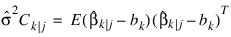
Computations for:
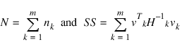
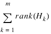
and Ck|j assume the variance-covariance matrices of the errors in the observation equation and state equation are known up to an unknown positive scalar multiplier, σ2. The maximum likelihood estimate of σ2 based on the observations y1, y2, …, ym, is given by:
where:
N and SS are the input/output arguments n and ss.
If σ2 is known, the Rks and Qks can be input as the variance-covariance matrices exactly. The earlier discussion is then simplified by letting σ2 = 1.
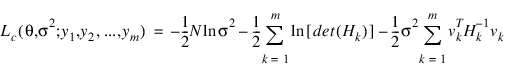
In practice, the matrices Tk, Qk, and Rk are generally not completely known. They may be known functions of an unknown parameter vector θ. In this case, KALMAN can be used in conjunction with an optimization program (see routine FMINV, PV-WAVE IMSL Mathematics Reference, Chapter 8, “Optimization”) to obtain a maximum likelihood estimate of θ. The natural logarithm of the likelihood function for y1, y2, ..., ym differs by no more than an additive constant from:
(Harvey 1981, page 14, equation 2.21).
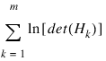
Here:
(stored in alndet) is the natural logarithm of the determinant of V where σ2V is the variance-covariance matrix of the observations.
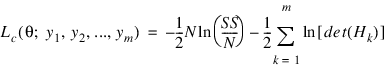
Minimization of -2L(θ, σ2; y1, y2, ..., ym) over all θ and σ2 produces maximum likelihood estimates. Equivalently, minimization of -2Lc(θ; y1, y2, ..., ym) where:
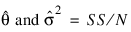
produces maximum likelihood estimates:
The minimization of -2Lc(θ; y1, y2, ..., ym) instead of -2L(θ, σ2; y1, y2, ..., ym), reduces the dimension of the minimization problem by one. The two optimization problems are equivalent since:
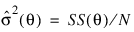
minimizes -2L(θ, σ2; y1, y2, ..., ym) for all θ, consequently:
can be substituted for σ2 in L(θ, σ2; y1, y2, …, ym) to give a function that differs by no more than an additive constant from Lc(θ; y1, y2, ..., ym).
The earlier discussion assumed Hk to be nonsingular. If Hk is singular, a modification for singular distributions described by Rao (1973, pages 527–528) is used. The changes in the preceding discussion are as follows:
1. Replace:
by a generalized inverse.
2. Replace det(Hk) by the product of the nonzero eigenvalues of Hk.
3. Replace N by:
Maximum likelihood estimation of parameters in the Kalman filter is discussed by Sallas and Harville (1988) and Harvey (1981, pages 111–113).
Example 1
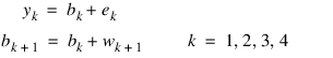
Routine KALMAN is used to compute the filtered estimates and one-step-ahead estimates for a scalar problem discussed by Harvey (1981, pages 116–117). The observation equation and state equation are given by:
where the eks are identically and independently distributed normal with mean 0 and variance σ2, the wks are identically and independently distributed normal with mean 0 and variance 4σ2, and b1 is distributed normal with mean 4 and variance 16σ2. Two invocations of KALMAN are needed for each time point in order to compute the filtered estimate and the one-step-ahead estimate. The first invocation does not use the keywords T_matrix and Q_matrix so that the prediction equations are skipped in the computations. The update equations are skipped in the computations in the second invocation.
This example also computes the one-step-ahead prediction errors. Harvey (1981, page 117) contains a misprint for the value v4 that he gives as 1.197. The correct value of v4 = 1.003 is computed by KALMAN.
Note that this example is in the form of a PV-WAVE procedure, with the output following the procedure.
PRO EX_KALMAN
z = 1
r = 1
q = 4
t = 1
b = 4
covb = 16
ydata = [4.4, 4, 3.5, 4.6]
n = 0
ss = 0
alndet = 0
format = '(2I4, 2F8.3, I4, 4F8.3)'
PRINT, ' k j b covb n ss alndet v covv'
FOR i=0L, 3 DO BEGIN
y = ydata(i)
; Update
KALMAN, b, covb, n, ss, alndet, Y = y, Z = Z, R = r, $
v = v, covv = covv
PRINT, i, i, b, covb, n, ss, alndet, v, covv, $
Format = format
; Predict
KALMAN, b, covb, n, ss, alndet, t_matrix = t, q = q
PRINT, i+1, i, b, covb, n, ss, alndet, v, covv, $
Format = format
END
END
This results in the following output:
k j b covb n ss alndet v covv
0 0 4.376 0.941 1 0.009 2.833 0.400 17.000
1 0 4.376 4.941 1 0.009 2.833 0.400 17.000
1 1 4.063 0.832 2 0.033 4.615 -0.376 5.941
2 1 4.063 4.832 2 0.033 4.615 -0.376 5.941
2 2 3.597 0.829 3 0.088 6.378 -0.563 5.832
3 2 3.597 4.829 3 0.088 6.378 -0.563 5.832
3 3 4.428 0.828 4 0.260 8.141 1.003 5.829
4 3 4.428 4.828 4 0.260 8.141 1.003 5.829
Version 2017.0
Copyright © 2017, Rogue Wave Software, Inc. All Rights Reserved.