iflag | Computed coefficient | |
–1 | 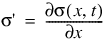 | |
0 | p(x) | |
1 | σ | |
2 | μ | |
3 | κ |
iflag | Computed coefficient | |
–1 | | |
0 | p(x) | |
1 | σ | |
2 | μ | |
3 | κ |

iflag | Computed boundary conditions | |
1 | Left end, x = xmin | |
2 | Right end, x = xmax |
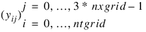
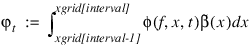
 for t = tgrid(i–1), i = 1, ..., ntgrid.
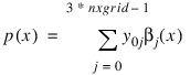
 for
for 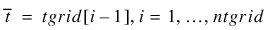
 for
for 
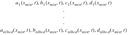
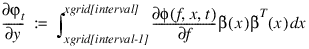
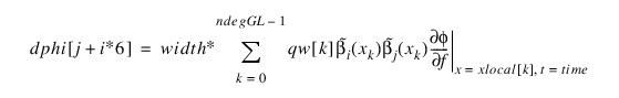
 at time point t=tgrid(i–1), i=1, ..., ntgrid and row 0 for the partials at t=0.
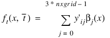
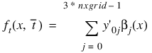
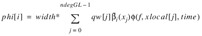
 at the Gauss-Legendre points xlocal. Setting
 and
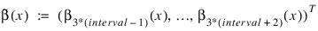
and  ,
,  is defined as:
i | time dependence of variable |
0 | σ' |
1 | σ |
2 | μ |
3 | κ |
4 | Left boundary conditions |
5 | Right boundary conditions |
6 | φ |
i | Entry in istate |
0 | Mass Matrix, M |
1 | Stiffness matrix, N |
2 | Bending matrix, R |
3 | Weighted mass, K |
4 | Left boundary condition data |
5 | Right boundary condition data |
6 | Forcing term |
i | nval(i) |
0 | Number of residual function evaluations of the DAE used in the model. |
1 | Number of factorizations of the differential matrix associated with solving the DAE. |
2 | Number of linear system solve steps using the differential matrix. |
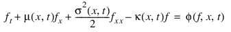
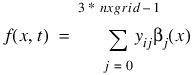
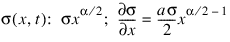
 , etc. The FEYNMAN_KAC function uses a finite element Galerkin method over the rectangle:
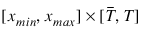


; These routines define the coefficients, payoff, boundary
; conditions and forcing term for American and European
; Options.
FUNCTION fkcfiv_put, x, tx, iflag, value
; The sigma value.
sigma=0.4
; Value of the interest rate and continuous dividend.
strike_price=10.0
interest_rate=0.1
dividend=0.0
zero=0.0
CASE iflag OF
0:BEGIN
; The payoff function.
value = MAX([strike_price - x, zero])
END
-1:BEGIN
; The coefficient derivative dsigma/dx.
value = sigma
END
1:BEGIN
; The coefficient sigma(x).
value = sigma*x
END
2:BEGIN
; The coefficient mu(x).
value = (interest_rate - dividend) * x
END
3:BEGIN
; The coefficient kappa(x).
value = interest_rate
END
ENDCASE
; Note that there is no time dependence.
iflag = 0L
RETURN,1
END
FUNCTION fkbcp_put, nbc, tx, iflag, val
CASE iflag OF
1:BEGIN
val(*) = 0.0
val(1) = 1.0
val(3) = -1.0
val(6) = 1.0
END
2:BEGIN
val(*) = 0.0
val(0) = 1.0
val(5) = 1.0
val(10) = 1.0
END
ENDCASE
; Note no time dependence.
iflag = 0
RETURN,1
END
FUNCTION fkforce_put, interval, ndeg, nxgrid, $
y, time, width, xlocal, $
qw, u, phi, dphi
COMMON f_kac_usr, usr_data
local=6
yl = FLTARR(local)
bf = FLTARR(local)
zero=0.0
one=1.0
index = INDGEN(local)
data = usr_data
yl = y(3*interval-3 + index)
phi(*) = zero
strike_price = data(0)
interest_rate = data(1)
value = data(2)
mu=2.0
; This is the local definition of the forcing term.
FOR j=1L, local DO BEGIN
FOR l=1L, ndeg DO BEGIN
bf(0) = u((l-1))
bf(1) = u((l-1)+ndeg)
bf(2) = u((l-1)+2*ndeg)
bf(3) = u((l-1)+6*ndeg)
bf(4) = u((l-1)+7*ndeg)
bf(5) = u((l-1)+8*ndeg)
rt = SUM(yl * bf)
rt = value/(rt + value - (strike_price-xlocal(l-1)))
phi(j-1) = phi(j-1) + (qw(l-1) * bf(j-1) * rt^mu)
ENDFOR
ENDFOR
phi = -phi * width*interest_rate*strike_price
; This is the local derivative matrix for the forcing term.
dphi(*) = zero
FOR j=1L, local DO BEGIN
FOR i=1L, local DO BEGIN
FOR l=1L, ndeg DO BEGIN
bf(0) = u((l-1))
bf(1) = u((l-1)+ndeg)
bf(2) = u((l-1)+2*ndeg)
bf(3) = u((l-1)+6*ndeg)
bf(4) = u((l-1)+7*ndeg)
bf(5) = u((l-1)+8*ndeg)
rt = SUM(yl * bf)
rt = one/(rt + value-(strike_price-xlocal(l-1)))
dphi(i-1+(j-1)*local) = dphi(i-1+(j-1)*local) + $
qw(l-1) * bf(i-1) * bf(j-1) $
* (rt^(mu+1.0))
ENDFOR
ENDFOR
ENDFOR
FOR i=0L, (local*local)-1 DO BEGIN
dphi(i) = mu * dphi(i) * width * value^mu * $
interest_rate * strike_price
ENDFOR
RETURN,1
END
PRO feynman_kac_ex1
; Compute American Option Premium for Vanilla Put.
COMMON f_kac_usr, usr_data
NXGRD = 61
NTGRD = 2
NV = 9
; The strike price.
KS = 10.0
; The sigma value.
sigma = 0.4
; Time values for the options.
nt = 2
time = [ 0.25, 0.5]
; Values of the underlying where evaluations are made.
xs = [ 0.0, 2.0, 4.0, 6.0, 8.0, 10.0, $
12.0, 14.0, 16.0 ]
; Value of the interest rate.
r = 0.1
; Values of the min and max underlying values modeled.
x_min=0.0
x_max=30.0
; Define parameters for the integration step.
nint=NXGRD-1
n=3*NXGRD
xgrid = FLTARR(NXGRD)
ye = FLTARR((NTGRD+1),3*NXGRD)
yeprime = FLTARR((NTGRD+1),3*NXGRD)
ya = FLTARR((NTGRD+1),3*NXGRD)
yaprime = FLTARR((NTGRD+1),3*NXGRD)
fe = FLTARR(NTGRD*NV)
fa = FLTARR(NTGRD*NV)
dx = 0.0
nlbcd = 2
nrbcd = 3
atol = 0.2e-2
; Array for user-defined data.
usr_data = FLTARR(3)
; Define an equally-spaced grid of points for the
; underlying price.
;
; Determine the increment between points (to be used later...)
dx = (x_max-x_min)/ nint
; Create the grid.
xgrid = INTERPOL([x_min,x_max], NXGRD)
Atol_Rtol = [ 0.5e-2, 0.5e-2 ]
; Set up the user data in the COMMON block for the user
; function(s).
usr_data = [KS, r, atol]
ret = FEYNMAN_KAC(nlbcd, nrbcd, xgrid, time, $
"fkcfiv_put", "fkbcp_put", ye, yeprime, $
ScalarAtolRtol=Atol_Rtol)
ret = FEYNMAN_KAC(nlbcd, nrbcd, xgrid, time, $
"fkcfiv_put", "fkbcp_put", ya, $
yaprime, Fcn_force="fkforce_put" , $
ScalarAtolRtol=Atol_Rtol)
; Evaluate solutions at vector of points XS(:), at each
; time value prior to expiration.
FOR i=0L, nt-1 DO BEGIN
fe(i*NV:(i*NV)+NV-1) = FEYNMAN_KAC_EVALUATE(xgrid, $
xs, ye((i+1),*))
fa(i*NV:(i*NV)+NV-1) = FEYNMAN_KAC_EVALUATE(xgrid, xs, $
ya((i+1),*))
ENDFOR
PRINT,'American Option Premium for Vanilla Put, ' + $
'3 and 6 Months Prior to Expiry'
PRINT," Number of equally spaced spline knots: ", NXGRD
PRINT," Number of unknowns: ", n
PRINT," Strike=",KS," sigma=",sigma," Interest Rate=",r
PRINT,""
PRINT,"Underlying European American"
FOR i=0L, NV-1 DO BEGIN
PRINT, xs(i), fe(i), fe(i+NV), fa(i), fa(i+NV), $
format='(5(f10.4))'
ENDFOR
PRINT,""
END
American Option Premium for Vanilla Put, 3 and 6 Months Prior to Expiry
Number of equally spaced spline knots: 61
Number of unknowns: 183
Strike= 10.0000, sigma= 0.400000, Interest Rate= 0.100000
Underlying European American
0.0000 9.7536 9.5134 10.0000 10.0000
2.0000 7.7537 7.5135 8.0000 8.0000
4.0000 5.7538 5.5150 6.0000 6.0000
6.0000 3.7619 3.5664 4.0000 4.0000
8.0000 1.9073 1.9170 2.0146 2.0880
10.0000 0.6518 0.8579 0.6768 0.9042
12.0000 0.1628 0.3392 0.1679 0.3526
14.0000 0.0374 0.1271 0.0374 0.1321
16.0000 0.0091 0.0477 0.0085 0.0499
FUNCTION fcn_fkcfiv, x, tx, iflag, value
COMMON f_kac_usr, usr_data
zero=0.0
half=0.5
data = usr_data
strike_price = data(0)
sigma = data(2)
alpha = data(3)
interest_rate = data(4)
dividend = data(5)
CASE iflag OF
0:BEGIN
; The payoff function.
value = (x - strike_price)>zero
END
-1:BEGIN
; The coefficient derivative d sigma/ dx.
value = half * alpha * sigma * x^(alpha*half-1.0)
END
1:BEGIN
; The coefficient sigma(x).
value = sigma * x^(alpha*half)
END
2:BEGIN
; The coefficient mu(x).
value = (interest_rate - dividend) * x
END
3:BEGIN
; The coefficient kappa(x).
value = interest_rate
END
ENDCASE
; Note that there is no time dependence.
iflag = 0
RETURN,1
END
FUNCTION fcn_fkbcp, nbc, tx, iflag, val
COMMON f_kac_usr, usr_data
data = usr_data
strike_price = data(0)
x_max = data(1)
interest_rate = data(4)
CASE iflag OF
1:BEGIN
val(*) = 0.0
val(0) = 1.0
val(5) = 1.0
val(10) = 1.0
; Note no time dependence at left end.
iflag = 0
END
2:BEGIN
df = EXP(interest_rate*tx)
val(*) = 0.0
val(0) = 1.0
val(3) = x_max - df*strike_price
val(5) = 1.0
val(7) = 1.0
val(10) = 1.0
END
ENDCASE
RETURN,1
END
PRO t_feynman_kac_ex2
COMMON f_kac_usr, usr_data
NXGRD = 121l
NTGRD = 3l
NV = 3l
; Compute Constant Elasticity of Variance Model for Vanilla Call
; The set of strike prices.
KS= [ 15.0, 20.0, 25.0]
; The set of sigma values.
sigma = [ 0.2, 0.3, 0.4]
; The set of model diffusion powers.
alpha = [2.0, 1.0, 0.0]
; Time values for the options.
nt = NTGRD
time = [ 1.0/12.0, 4.0/12.0, 7.0/12.0 ]
; Values of the underlying where evaluations are made.
xs = [ 19.0, 20.0, 21.0 ]
; Value of the interest rate and continuous dividend.
r=0.05
dividend=0.0
; Values of the min and max underlying values modeled.
x_min=0.0
x_max=60.0
; Define parameters for the integration step.
nint = NXGRD-1
n = 3*NXGRD
xgrid = FLTARR(NXGRD)
y = FLTARR((NTGRD+1)*3*NXGRD)
yprime = FLTARR((NTGRD+1)*3*NXGRD)
f = FLTARR(NTGRD*NV)
dx = 0.0
; Number of left/right boundary conditions.
nlbcd = 3L
nrbcd = 3L
usr_data = FLTARR(6)
; Define equally-spaced grid of points for the underlying price.
xgrid = INTERPOL([x_min,x_max], NXGRD)
PRINT,"Constant Elasticity of Variance Model for Vanilla Call"
PRINT,"Interest Rate: ",r," Continuous Dividend: ", dividend
PRINT,"Minimum and Maximum Prices of Underlying: ", $
STRING(x_min,Format="(f6.2)"), " ",$
STRING(x_max ,Format="(f6.2)")
PRINT,"Number of equally spaced spline knots:",NXGRD-1
PRINT,"Number of unknowns:",n
PRINT,""
PRINT,"Time in Years Prior to Expiration: ", $
STRING(time(0),Format="(f7.4)"), " ",$
STRING(time(1),Format="(f7.4)"), " ",$
STRING(time(2),Format="(f7.4)")
PRINT,"Option valued at Underlying Prices: ", $
STRING(xs(0),Format="(f5.2)"), " ",$
STRING(xs(1),Format="(f5.2)"), " ",$
STRING(xs(2),Format="(f5.2)")
PRINT,""
FOR i1=1L, 3 DO BEGIN ; Loop over power.
FOR i2=1L, 3 DO BEGIN ; Loop over volatility.
FOR i3=1L, 3 DO BEGIN ; Loop over strike price.
; Pass data through into evaluation routines.
usr_data(0) = KS(i3-1)
usr_data(1) = x_max
usr_data(2) = sigma(i2-1)
usr_data(3) = alpha(i1-1)
usr_data(4) = r
usr_data(5) = dividend
ret = FEYNMAN_KAC(nlbcd, nrbcd, xgrid, time, $
"fcn_fkcfiv", "fcn_fkbcp", y, yprime)
; Evaluate solution at vector of points xs, at each
; time Value prior to expiration.
FOR i=0L, NTGRD-1 DO $
f(i*NV:(i*NV)+NV-1) = $
FEYNMAN_KAC_EVALUATE(xgrid, xs, REFORM(y((i+1),*)))
outstr = "Strike="+STRING(KS(i3-1),Format="(f6.2)")+ $
" Sigma="+STRING(sigma(i2-1),Format="(f6.2)")+ $
" Alpha="+STRING(alpha(i1-1),Format="(f6.2)")
PRINT, outstr
FOR i=0L, NV-1 DO BEGIN
outstr = " Call Option Values "+ $
STRING(f(i),Format="(f7.4)") + " "+ $
STRING(f(NV+i),Format="(f7.4)") + " "+ $
STRING(f(2*NV+i),Format="(f7.4)")
PRINT, outstr
ENDFOR
ENDFOR
ENDFOR
ENDFOR
END
Constant Elasticity of Variance Model for Vanilla Call
Interest Rate: 0.0500000 Continuous Dividend: 0.00000
Minimum and Maximum Prices of Underlying: 0.00 60.00
Number of equally spaced spline knots: 120
Number of unknowns: 363
Time in Years Prior to Expiration: 0.0833 0.3333 0.5833
Option valued at Underlying Prices: 19.00 20.00 21.00
Strike= 15.00 Sigma= 0.20 Alpha= 2.00
Call Option Values 4.0624 4.2575 4.4729
Call Option Values 5.0624 5.2506 5.4490
Call Option Values 6.0624 6.2486 6.4385
Strike= 20.00 Sigma= 0.20 Alpha= 2.00
Call Option Values 0.1310 0.5956 0.9698
Call Option Values 0.5029 1.0889 1.5100
Call Option Values 1.1980 1.7484 2.1751
Strike= 25.00 Sigma= 0.20 Alpha= 2.00
Call Option Values 0.0000 0.0113 0.0744
Call Option Values 0.0000 0.0373 0.1615
Call Option Values 0.0007 0.1026 0.3132
Strike= 15.00 Sigma= 0.30 Alpha= 2.00
Call Option Values 4.0639 4.3397 4.6618
Call Option Values 5.0626 5.2945 5.5783
Call Option Values 6.0624 6.2709 6.5238
Strike= 20.00 Sigma= 0.30 Alpha= 2.00
Call Option Values 0.3109 1.0275 1.5500
Call Option Values 0.7323 1.5422 2.1024
Call Option Values 1.3765 2.1690 2.7385
Strike= 25.00 Sigma= 0.30 Alpha= 2.00
Call Option Values 0.0006 0.1111 0.3542
Call Option Values 0.0037 0.2169 0.5547
Call Option Values 0.0182 0.3857 0.8222
Strike= 15.00 Sigma= 0.40 Alpha= 2.00
Call Option Values 4.0755 4.5138 4.9674
Call Option Values 5.0661 5.4201 5.8324
Call Option Values 6.0634 6.3578 6.7298
Strike= 20.00 Sigma= 0.40 Alpha= 2.00
Call Option Values 0.5116 1.4645 2.1292
Call Option Values 0.9623 1.9957 2.6951
Call Option Values 1.5815 2.6110 3.3236
Strike= 25.00 Sigma= 0.40 Alpha= 2.00
Call Option Values 0.0083 0.3284 0.7785
Call Option Values 0.0284 0.5165 1.0654
Call Option Values 0.0812 0.7686 1.4104
Strike= 15.00 Sigma= 0.20 Alpha= 1.00
Call Option Values 4.0624 4.2479 4.4312
Call Option Values 5.0624 5.2479 5.4312
Call Option Values 6.0624 6.2479 6.4312
Strike= 20.00 Sigma= 0.20 Alpha= 1.00
Call Option Values 0.0000 0.0226 0.1049
Call Option Values 0.1495 0.4107 0.6485
Call Option Values 1.0832 1.3314 1.5773
Strike= 25.00 Sigma= 0.20 Alpha= 1.00
Call Option Values 0.0000 -0.0000 0.0000
Call Option Values -0.0000 -0.0000 0.0000
Call Option Values -0.0000 0.0000 0.0000
Strike= 15.00 Sigma= 0.30 Alpha= 1.00
Call Option Values 4.0624 4.2479 4.4312
Call Option Values 5.0624 5.2479 5.4312
Call Option Values 6.0624 6.2479 6.4312
Strike= 20.00 Sigma= 0.30 Alpha= 1.00
Call Option Values 0.0016 0.0785 0.2204
Call Option Values 0.1979 0.4997 0.7541
Call Option Values 1.0836 1.3443 1.6022
Strike= 25.00 Sigma= 0.30 Alpha= 1.00
Call Option Values -0.0000 0.0000 0.0000
Call Option Values -0.0000 0.0000 0.0000
Call Option Values -0.0000 0.0000 0.0005
Strike= 15.00 Sigma= 0.40 Alpha= 1.00
Call Option Values 4.0624 4.2477 4.4310
Call Option Values 5.0624 5.2477 5.4309
Call Option Values 6.0624 6.2477 6.4309
Strike= 20.00 Sigma= 0.40 Alpha= 1.00
Call Option Values 0.0084 0.1542 0.3443
Call Option Values 0.2482 0.5943 0.8729
Call Option Values 1.0871 1.3790 1.6584
Strike= 25.00 Sigma= 0.40 Alpha= 1.00
Call Option Values 0.0000 0.0000 0.0001
Call Option Values 0.0000 0.0000 0.0008
Call Option Values 0.0000 0.0004 0.0066
Strike= 15.00 Sigma= 0.20 Alpha= 0.00
Call Option Values 4.0627 4.2478 4.4312
Call Option Values 5.0623 5.2479 5.4311
Call Option Values 6.0623 6.2479 6.4312
Strike= 20.00 Sigma= 0.20 Alpha= 0.00
Call Option Values 0.0001 0.0001 0.0002
Call Option Values 0.0816 0.3316 0.5748
Call Option Values 1.0818 1.3308 1.5748
Strike= 25.00 Sigma= 0.20 Alpha= 0.00
Call Option Values 0.0000 -0.0000 -0.0000
Call Option Values 0.0000 -0.0000 -0.0000
Call Option Values -0.0000 0.0000 -0.0000
Strike= 15.00 Sigma= 0.30 Alpha= 0.00
Call Option Values 4.0625 4.2479 4.4312
Call Option Values 5.0623 5.2479 5.4312
Call Option Values 6.0624 6.2479 6.4312
Strike= 20.00 Sigma= 0.30 Alpha= 0.00
Call Option Values 0.0000 -0.0000 0.0029
Call Option Values 0.0895 0.3326 0.5753
Call Option Values 1.0826 1.3306 1.5749
Strike= 25.00 Sigma= 0.30 Alpha= 0.00
Call Option Values 0.0000 -0.0000 0.0000
Call Option Values 0.0000 -0.0000 -0.0000
Call Option Values 0.0000 -0.0000 -0.0000
Strike= 15.00 Sigma= 0.40 Alpha= 0.00
Call Option Values 4.0624 4.2479 4.4312
Call Option Values 5.0623 5.2479 5.4312
Call Option Values 6.0624 6.2479 6.4312
Strike= 20.00 Sigma= 0.40 Alpha= 0.00
Call Option Values -0.0000 0.0001 0.0111
Call Option Values 0.0985 0.3383 0.5781
Call Option Values 1.0830 1.3306 1.5749
Strike= 25.00 Sigma= 0.40 Alpha= 0.00
Call Option Values 0.0000 0.0000 0.0000
Call Option Values 0.0000 -0.0000 0.0000
Call Option Values 0.0000 -0.0000 0.0000
PRO t_feynman_kac_ex3
COMMON f_kac_usr, usr_data
NXGRD = 61l
NTGRD = 2l
NV = 12l
; The strike price.
KS1 = 10.0
; The spread value.
KS2 = 15.0
; The Bet for the Cash-or-Nothing Call.
bet = 2.0
; The sigma value.
sigma = 0.4
; Time values for the options.
time = [0.25, 0.5]
; Values of the underlying where evaluations are made.
xs = FLTARR(NV)
; Value of the interest rate and continuous dividend.
r = 0.1
dividend=0.0
; Values of the min and max underlying values modeled.
x_min=0.0
x_max=30.0
; Define parameters for the integration step.
nint = NXGRD-1
n = 3*NXGRD
xgrid = FLTARR(NXGRD)
yb = FLTARR((NTGRD+1)*3*NXGRD)
ybprime = FLTARR((NTGRD+1)*3*NXGRD)
yv = FLTARR((NTGRD+1)*3*NXGRD)
yvprime = FLTARR((NTGRD+1)*3*NXGRD)
fb = FLTARR(NTGRD*NV)
fv = FLTARR(NTGRD*NV)
; Number of left/right boundary conditions.
nlbcd = 3l
nrbcd = 3l
; Structure for the evaluation routines.
usr_data = { , $idope:I32ARR(1), $
rdope:FLTARR(7) $
}
; Define an equally-spaced grid of points for the underlying
; price.
xgrid = INTERPOL([x_min, x_max], NXGRD)
tmp = FINDGEN(NV)
xs = 2.0+(tmp*2.0)
usr_data.rdope(0) = KS1
usr_data.rdope(1) = bet
usr_data.rdope(2) = KS2
usr_data.rdope(3) = x_max
usr_data.rdope(4) = sigma
usr_data.rdope(5) = r
usr_data.rdope(6) = dividend
; Flag the difference in payoff functions
; 1 for the Bet, 2 for the Vertical Spread.
usr_data.idope(0) = 1
ret = FEYNMAN_KAC(nlbcd, nrbcd, $
xgrid, time, "fkcfiv_call", $
"fkbcp_call", yb, ybprime)
usr_data.idope(0) = 2
ret = FEYNMAN_KAC(nlbcd, nrbcd, $
xgrid, time, "fkcfiv_call",$
"fkbcp_call", yv, yvprime)
; Evaluate solutions at vector of points XS(:), at
; each time value prior to expiration.
FOR i=0L, NTGRD-1 DO BEGIN
fb(i*NV:(i*NV)+NV-1) = FEYNMAN_KAC_EVALUATE(xgrid, $
xs, REFORM(yb((i+1),*)))
fv(i*NV:(i*NV)+NV-1) = FEYNMAN_KAC_EVALUATE(xgrid, $
xs, REFORM(yv((i+1),*)))
ENDFOR
PRINT,""
PRINT,"European Option Value for A Bet"
PRINT," and a Vertical Spread, 3 and 6 Months Prior to Expiry"
PRINT," Number of equally spaced spline knots: ", $
STRTRIM(NXGRD,2)
PRINT," Number of unknowns: ",STRTRIM(n,2)
PRINT," Strike=", STRING(KS1,Format="(f5.2)"),$
" Sigma=",STRING(sigma,Format="(f5.2)"),$
" Interest Rate=",STRING(r,Format="(f5.2)")
PRINT," Bet=",STRING(bet,Format="(f5.2)"), $
" Spread Value= ",STRING(KS2,Format="(f5.2)")
PRINT,""
PRINT," Underlying A Bet Vertical Spread
FOR i=0L, NV-1 DO BEGIN
PRINT," ",STRING(xs(i),Format="(f9.4)")," ", $
STRING(fb(i),Format="(f9.4)"), " ",$
STRING(fb(i+NV),Format="(f9.4)")," ",$
STRING(fv(i),Format="(f9.4)"), " ",$
STRING(fv(i+NV),Format="(f9.4)")
ENDFOR
END
; These routines define the coefficients, payoff, boundary
; conditions and forcing term for American and European Options.
FUNCTION fkcfiv_call, x, tx, iflag, value
COMMON f_kac_usr, usr_data
zero=0.0
data = usr_data
data_real = data.rdope
data_int = data.idope
strike_price = data_real(0)
bet = data_real(1)
spread = data_real(2)
sigma = data_real(4)
interest_rate = data_real(5)
dividend = data_real(6)
CASE iflag OF
0:BEGIN
; The payoff function - Use flag passed to decide which.
CASE data_int(0) OF
1:BEGIN
; After reaching the strike price the payoff
; jumps from zero to the bet value.
value = zero
IF (x GT strike_price) THEN value = bet
END
2:BEGIN
; Function is zero up to strike price.
; Then linear between strike price and spread.
; Then has constant value Spread-Strike Price
; after the value Spread.
value = ((x-strike_price)>zero) - (x-spread>zero)
END
ENDCASE
END
-1:BEGIN
; The coefficient derivative d sigma/ dx.
value = sigma
END
1:BEGIN
; The coefficient sigma(x).
value = sigma*x
END
2:BEGIN
; The coefficient mu(x).
value = (interest_rate - dividend)*x
END
3:BEGIN
; The coefficient kappa(x).
value = interest_rate
END
ENDCASE
; Note that there is no time dependence.
iflag = 0
RETURN,1
END
FUNCTION fkbcp_call, nbc, tx, iflag, val
COMMON f_kac_usr, usr_data
data = usr_data
data_int = data.idope
data_real = data.rdope
strike_price = data_real(0)
bet = data_real(1)
spread = data_real(2)
interest_rate = data_real(5)
CASE iflag OF
1:BEGIN
val(*) = 0.0
val(0) = 1.0
val(5) = 1.0
val(10) = 1.0
; Note no time dependence in case (1) for IFLAG.
iflag = 0
END
2:BEGIN
; This is the discount factor using the risk-free
; interest rate.
df = EXP(interest_rate*tx)
; Use flag passed to decide on boundary condition.
CASE data_int(0) OF
1:BEGIN
val(*) = 0.0
val(0) = 1.0
val(3) = bet*df
END
2:BEGIN
val(*) = 0.0
val(0) = 1.0
val(3) = (spread-strike_price)*df
END
ENDCASE
val(5) = 1.0
val(10) = 1.0
END
ENDCASE
RETURN,1
END
European Option Value for A Bet and a Vertical Spread, 3 and 6 Months Prior to Expiry Number of equally spaced spline knots: 61 Number of unknowns: 183 Strike=10.00 Sigma= 0.40 Interest Rate= 0.10 Bet= 2.00 Spread Value= 15.00 Underlying A Bet Vertical Spread 2.0000 0.0000 0.0000 0.0000 0.0000 4.0000 0.0000 0.0014 0.0000 0.0006 6.0000 0.0110 0.0722 0.0039 0.0447 8.0000 0.2691 0.4305 0.1479 0.3831 10.0000 0.9948 0.9781 0.8909 1.1927 12.0000 1.6094 1.4287 2.1911 2.2273 14.0000 1.8655 1.6923 3.4254 3.1552 16.0000 1.9337 1.8177 4.2263 3.8263 18.0000 1.9476 1.8700 4.6264 4.2492 20.0000 1.9501 1.8903 4.7911 4.4921 22.0000 1.9505 1.8979 4.8497 4.6231 24.0000 1.9506 1.9007 4.8684 4.6909PRO t_feynman_kac_ex4
COMMON f_kac_usr, usr_data
; Compute value of a Convertible Bond.
NXGRD = 61
NTGRD = 2
NV = 13
; The face value.
KS = 1.0e0
; The sigma or volatility value.
sigma = 0.25e0
; Time values for the options.
time = [ 0.5, 1.0 ]
; Values of the underlying where evaluation are made.
xs = FLTARR(NV)
; Value of the interest rate, continuous dividend and factor.
r = 0.1
dividend=0.02
factor = 1.125
; Values of the min and max underlying values modeled.
x_min = 0.0
x_max = 4.0
; Define parameters for the integration step.
nint = NXGRD-1
n = 3*NXGRD
xgrid = FLTARR(NXGRD)
y = FLTARR((NTGRD+1)*3*NXGRD)
yprime = FLTARR((NTGRD+1)*3*NXGRD)
f = FLTARR((NTGRD+1)*NV)
; Array for user-defined data.
usr_data = FLTARR(8)
; Number of left/right boundary conditions.
nlbcd = 3l
nrbcd = 3l
; Define an equally-spaced grid of points for the
; underlying price.
dx = (x_max-x_min)/(nint)
xgrid = INTERPOL([x_min, x_max], NXGRD)
tmp = FINDGEN(NV)
xs = tmp*0.25
; Pass the data for evaluation.
usr_data(0) = KS
usr_data(1) = x_max
usr_data(2) = sigma
usr_data(3) = r
usr_data(4) = dividend
usr_data(5) = factor
; Use a pure absolute error tolerance for the integration.
atol = 1.0e-3
usr_data(6) = atol
; Compute value of convertible bond.
ret = FEYNMAN_KAC(nlbcd, nrbcd, xgrid, time, $
"fkcfiv_cbond", "fkbcp_cbond", y, yprime, $
Fcn_fkinit="fkinit_cbond", $
Fcn_force="fkforce_cbond", $
ScalarAtolRtol=[1.0e-3, 0.0e0] )
; Evaluate and display solutions at vector of points XS(:),
; at each time value prior to expiration.
FOR i=0L, NTGRD DO BEGIN
f(i*NV:(i*NV)+NV-1) = FEYNMAN_KAC_EVALUATE (xgrid, xs, REFORM(y(i,*)))
ENDFOR
PRINT,"Convertible Bond Value, 0+, 6 and 12 Months Prior"+ $
" to Expiry"
PRINT," Number of equally spaced spline knots: ", $
STRTRIM(NXGRD,2)
PRINT," Number of unknowns:",STRTRIM(n,2)
PRINT," Strike= ",STRING(KS,Format="(f5.2)"), $
" Sigma= ",STRING(sigma,Format="(f5.2)")
PRINT," Interest Rate= ",STRING(r,Format="(f5.2)"), $
" Dividend= ",STRING(dividend,Format="(f5.2)"), $
" Factor= ",STRING(factor,Format="(f6.3)")
PRINT,""
PRINT,"Underlying Bond Value"
FOR i=0L, NV-1 DO BEGIN
PRINT," ",STRING(xs(i),Format="(f8.4)")," ", $
STRING(f(i),Format="(f8.4)")," ", $
STRING(f(i+NV),Format="(f8.4)")," ", $
STRING(f(i+2*NV),Format="(f8.4)")
ENDFOR
END
; These routines define the coefficients, payoff,
; boundary conditions and forcing term.
FUNCTION fkcfiv_cbond, x, tx, iflag, value
COMMON f_kac_usr, usr_data
zero=0.0
data = usr_data
strike_price = data(0)
sigma = data(2)
interest_rate = data(3)
dividend = data(4)
factor = data(5)
CASE iflag OF
0:BEGIN
; The payoff function.
value = (factor * x)>strike_price
END
-1:BEGIN
; The coefficient derivative d sigma/ dx.
value = sigma
END
1:BEGIN
; The coefficient sigma(x).
value = sigma*x
END
2:BEGIN
; The coefficient mu(x).
value = (interest_rate - dividend) * x
END
3:BEGIN
; The coefficient kappa(x).
value = interest_rate
END
ENDCASE
; Note that there is no time dependence.
iflag = 0
RETURN,1
END
FUNCTION fkbcp_cbond, nbc, tx, iflag, val
COMMON f_kac_usr, usr_data
data = usr_data
CASE iflag OF
1:BEGIN
strike_price = data(0)
interest_rate = data(3)
dp = strike_price * EXP(tx*interest_rate)
val(*) = 0.0
val(0) = 1.0
val(3) = dp
val(5) = 1.0
val(10) = 1.0
END
2:BEGIN
x_max = data(1)
factor = data(5)
val(*) = 0.0
val(0) = 1.0
val(3) = factor*x_max
val(5) = 1.0
val(7) = factor
val(10) = 1.0
; Note no time dependence.
iflag = 0
END
ENDCASE
RETURN,1
END
FUNCTION fkforce_cbond, interval, ndeg, nxgrid, y, $
time, width, xlocal, qw, $
u, phi, dphi
COMMON f_kac_usr, usr_data
local=6
yl = FLTARR(local)
bf = FLTARR(local)
zero=0.e0
one=1.0e0
data = usr_data
phi(*) = zero
dphi(*) = zero
yl = y((3*interval)-3+INDGEN(local))
value = data(6)
strike_price = data(0)
interest_rate = data(3)
factor = data(5)
mu = 2.0
; This is the local definition of the forcing term.
; It "forces" the constraint f >= factor*x.
FOR j=1L, local DO BEGIN
FOR l=1L, ndeg DO BEGIN
bf(0) = u((l-1))
bf(1) = u((l-1)+ndeg)
bf(2) = u((l-1)+2*ndeg)
bf(3) = u((l-1)+6*ndeg)
bf(4) = u((l-1)+7*ndeg)
bf(5) = u((l-1)+8*ndeg)
rt = SUM(yl * bf)
rt = value/(rt + value - factor * xlocal(l-1))
phi(j-1) = phi(j-1) + qw(l-1) * bf(j-1) * rt^mu
ENDFOR
ENDFOR
phi = (-phi)*width*factor*strike_price
; This is the local derivative matrix for the forcing term
FOR j=1L, local DO BEGIN
FOR i=1L, local DO BEGIN
FOR l=1L, ndeg DO BEGIN
bf(0) = u((l-1))
bf(1) = u((l-1)+ndeg)
bf(2) = u((l-1)+2*ndeg)
bf(3) = u((l-1)+6*ndeg)
bf(4) = u((l-1)+7*ndeg)
bf(5) = u((l-1)+8*ndeg)
rt = SUM(yl * bf)
rt = one/(rt + value - factor * xlocal(l-1))
dphi(i-1+(j-1)*local) = $
dphi(i-1+(j-1)*local)+qw(l-1) * bf(i-1) * $
bf(j-1) * ((value*rt)^mu) * rt
ENDFOR
ENDFOR
ENDFOR
dphi = dphi *(-mu) * width * factor * strike_price
RETURN,1
END
FUNCTION fkinit_cbond, nxgrid, ntgrid, xgrid, tgrid, $
time, yprime, y, atol, rtol
COMMON f_kac_usr, usr_data
data = usr_data
IF time EQ 0.0 THEN BEGIN
; Set initial data precisely.
FOR i=1L, nxgrid DO BEGIN
IF (xgrid(i-1) * data(5)) LT data(0) THEN BEGIN
y(3*i-3) = data(0)
y(3*i-2) = 0.0
y(3*i-1) = 0.0
ENDIF ELSE BEGIN
y(3*i-3) = xgrid(i-1) * data(5)
y(3*i-2) = data(5)
y(3*i-1) = 0.0
ENDELSE
ENDFOR
ENDIF
RETURN,1
END
Convertible Bond Value, 0+, 6 and 12 Months Prior to Expiry
Number of equally spaced spline knots: 61
Number of unknowns:183
Strike= 1.00 Sigma= 0.25
Interest Rate= 0.10 Dividend= 0.02 Factor= 1.125
Underlying Bond Value
0.0000 1.0000 0.9512 0.9048
0.2500 1.0000 0.9512 0.9049
0.5000 1.0000 0.9513 0.9065
0.7500 1.0000 0.9737 0.9605
1.0000 1.1250 1.1416 1.1464
1.2500 1.4062 1.4117 1.4121
1.5000 1.6875 1.6922 1.6922
1.7500 1.9688 1.9731 1.9731
2.0000 2.2500 2.2540 2.2540
2.2500 2.5312 2.5349 2.5349
2.5000 2.8125 2.8160 2.8160
2.7500 3.0938 3.0970 3.0970
3.0000 3.3750 3.3781 3.3781