MULTIVARIATE_NORMAL_CDF Function (PV-WAVE Advantage)
Evaluates the cumulative distribution function for the multivariate normal distribution.
Usage
result = MULTIVARIATE_NORMAL_CDF (h, mean, sigma)
Input Parameters
h—Array of length
k containing the upper bounds for calculating the cumulative distribution function,

. Where
k is the number of variates in the multivariate normal distribution.
mean—Array of length
k containing the mean of the multivariate normal distribution, i.e.,
. Where
k is the number of variates in the multivariate normal distribution.
sigma—A 2D array of size
k by
k containing the positive definite symmetric matrix of correlations or of variances and covariances for the multivariate normal distribution, i.e.,
. Where
k is the number of variates in the multivariate normal distribution.
Returned Value
result—The value of the cumulative distribution function for a multivariate normal random variable,
.
Input Keywords
Double—If present and nonzero, then double precision is used.
Print—If present and nonzero, this option turns on printing of the intermediate computations. By default, intermediate computations are not printed.
Err_abs—The absolute accuracy requested for the calculated cumulative probability. Default: Err_abs = 1.0e–3.
Err_rel—The relative accuracy desired. Default: Err_rel = 1.0e–5.
Tolerance—The minimum value for the smallest eigenvalue of sigma. If the smallest eigenvalue is less than tolerance, then the terminal error IMSLS_SIGMA_SINGULAR is issued. Default: Tolerance=ε, where ε is the machine precision.
Max_evals—The maximum number of function evaluations allowed. If this limit is exceeded, the IMSLS_MAX_EVALS_EXCEEDED warning message is issued and the optimization terminates. Default: Max_evals = 1000*k.
Random_seed—The value of the random seed used for generating quadrature points. By using different seeds on different calls to this routine, slightly different answers will be obtained in the digits beyond the estimated error. If Random_seed = 0, then the seed is set to the value of the system clock which will automatically generate slightly different answers for each call. Default: Random_seed = 7919.
Output Keywords
Err_est—The estimated error.
Discussion
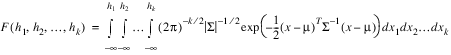
Function MULTIVARIATE_NORMAL_CDF evaluates the cumulative distribution function
F of a multivariate normal distribution with
and
. The input arrays
mean and
sigma are used as the values for
μ and
∑, respectively. The formula for the CDF calculation is given by the multiple integral described in Johnson and Kotz (1972):
∑ must be positive definite, i.e. |
∑| > 0. If
k = 2 or
k > 2 the
NORMALCDF Function (PV-WAVE Advantage) and
BINORMALCDF Function (PV-WAVE Advantage) are used for this calculation.
In the special case of equal correlations, the above integral is transformed into a univariate integral using the transformation developed by Dunnett and Sobel(1955). This produces very accurate and fast calculations even for a large number of variates.
If k >2 and the correlations are not equal, the Cholesky decomposition transformation described by Genz(1992) is used (with permission from the author). This transforms the problem into a definite integral involving k–1 variables which is solved numerically using randomized Korobov rules if k ≤ 100, see Cranley and Patterson (1976) and Keast (1973); otherwise, the integral is solved using quasi-random Richtmeyer points described in Davis and Rabinowitz (1984).
Example 1
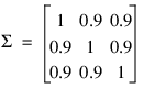
This example evaluates the cumulative distribution function for a trivariate normal random variable. There are three calculations. The first calculation is of F(1.96, 1.96, 1.96) for a trivariate normal variable with μ = {0, 0, 0}, and:
In this case, MULTIVARIATE_NORMAL_CDF calculates F(1.96, 1.96, 1.96) = 0.958179.
The second calculation involves a trivariate variable with the same correlation matrix as the first calculation but with a mean of μ = {0, 1, –1}. This is the same distribution as the first example shifted by the mean. The calculation of F(1.96, 2.96, 0.96) verifies that this probability is equal to the same value as reported for the first case.
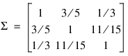
The last calculation is the same calculation reported in Genz (1992) for a trivariate normal random variable with μ = {0, 0, 0} and:
In this example the calculation of F(1, 4, 2) = 0.827985.
PRO t_multivariate_normal_cdf_ex1
bounds1 = [1.96, 1.96, 1.96]
bounds2 = [1.96, 2.96, 0.96]
bounds3 = [1.0, 4.0, 2.0]
mean1 = [0.0, 0.0, 0.0]
mean2 = [0.0, 1.0, -1.0]
stdev1 = [1.0, 0.9, 0.9,$
0.9, 1.0, 0.9,$
0.9, 0.9, 1.0]
stdev2 = [1.0, 0.6, 1.0/3.0,$
0.6, 1.0, 11.0/15.0,$
1.0/3.0, 11.0/15.0, 1.0]
PRINT,"Mean Vector: "
PRINT,STRTRIM(STRING(mean1(0),Format="(I)"),2)," ",$
STRTRIM(STRING(mean1(1),Format="(I)"),2)," ",$
STRTRIM(STRING(mean1(2),Format="(I)"),2)
PRINT,""
PRINT,"Correlation Matrix"
FOR i=0L, 8, 3 DO BEGIN
PRINT,STRTRIM(STRING(stdev1(i),Format="(f3.1)"),2)," ",$
STRTRIM(STRING(stdev1(i+1),Format="(f3.1)"),2)," ",$
STRTRIM(STRING(stdev1(i+2),Format="(f3.1)"),2)
ENDFOR
f = MULTIVARIATE_NORMAL_CDF(bounds1, mean1, stdev1 )
PRINT,""
PRINT,"F(X1< ",STRTRIM(STRING(bounds1(0),Format="(f6.4)"),2),$
", X2<",STRTRIM(STRING(bounds1(1),Format="(f6.4)"),2),$
", X3<",STRTRIM(STRING(bounds1(2),Format="(f6.4)"),2),$
") = ",STRTRIM(STRING(f,Format="(f10.6)"),2)
PRINT,""
PRINT,"Mean Vector: "
PRINT,STRTRIM(STRING(mean2(0),Format="(I)"),2)," ",$
STRTRIM(STRING(mean2(1),Format="(I)"),2)," ",$
STRTRIM(STRING(mean2(2),Format="(I)"),2)
PRINT,""
PRINT,"Correlation Matrix"
FOR i=0L, 8, 3 DO BEGIN
PRINT,STRTRIM(STRING(stdev1(i),Format="(f3.1)"),2)," ",$
STRTRIM(STRING(stdev1(i+1),Format="(f3.1)"),2)," ",$
STRTRIM(STRING(stdev1(i+2),Format="(f3.1)"),2)
ENDFOR
f = MULTIVARIATE_NORMAL_CDF(bounds2, mean2, stdev1 )
PRINT,""
PRINT,"F(X1< ",STRTRIM(STRING(bounds2(0),Format="(f6.4)"),2),$
", X2<",STRTRIM(STRING(bounds2(1),Format="(f6.4)"),2),$
", X3<",STRTRIM(STRING(bounds2(2),Format="(f6.4)"),2),$
") = ",STRTRIM(STRING(f,Format="(f10.6)"),2)
PRINT,""
PRINT,"Mean Vector: "
PRINT,STRTRIM(STRING(mean1(0),Format="(I)"),2)," ",$
STRTRIM(STRING(mean1(1),Format="(I)"),2)," ",$
STRTRIM(STRING(mean1(2),Format="(I)"),2)
PRINT,""
PRINT,"Correlation Matrix"
FOR i=0L, 8, 3 DO BEGIN
PRINT,STRTRIM(STRING(stdev2(i),Format="(f3.1)"),2)," ",$
STRTRIM(STRING(stdev2(i+1),Format="(f3.1)"),2)," ",$
STRTRIM(STRING(stdev2(i+2),Format="(f3.1)"),2)
ENDFOR
f = MULTIVARIATE_NORMAL_CDF(bounds3, mean1, stdev2 )
PRINT,""
PRINT,"F(X1< ",STRTRIM(STRING(bounds3(0),Format="(f6.4)"),2),$
", X2<",STRTRIM(STRING(bounds3(1),Format="(f6.4)"),2),$
", X3<",STRTRIM(STRING(bounds3(2),Format="(f6.4)"),2),$
") = ",STRTRIM(STRING(f,Format="(f10.6)"),2)
PRINT,""
END
Output
Mean Vector:
0 0 0
Correlation Matrix
1.0 0.9 0.9
0.9 1.0 0.9
0.9 0.9 1.0
RESULT FLOAT = 0.958179
F(X1< 1.9600, X2<1.9600, X3<1.9600) = 0.958179
Mean Vector:
0 1 -1
Correlation Matrix
1.0 0.9 0.9
0.9 1.0 0.9
0.9 0.9 1.0
RESULT FLOAT = 0.958179
F(X1< 1.9600, X2<2.9600, X3<0.9600) = 0.958179
Mean Vector:
0 0 0
Correlation Matrix
1.0 0.6 0.3
0.6 1.0 0.7
0.3 0.7 1.0
RESULT FLOAT = 0.827985
F(X1< 1.0000, X2<4.0000, X3<2.0000) = 0.827985
Example 2
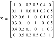
This example illustrates the calculation of the CDF for a multivariate normal distribution with a mean of μ = {1, 0, –1, 0, 1, –1}, and a correlation matrix of:
The keyword Print is used to illustrate the type of intermediate output available from this function. This routine sorts the variables by the limits for the CDF calculation specified in x. This improves the accuracy of the calculations, see Genz (1992). In this case, F(X1 < 1, X2 < 2.5, X3 < 2, X4 < 0.5, X5 < 0, X6 < 0.8) = 0.087237 with an estimated error of 8.7e–05.
By increasing the correlation of X2 and X3 from 0.1 to 0.7, the correlation matrix becomes singular. This routine checks for this condition and issues an error when sigma is not symmetric or positive definite.
PRO t_multivariate_normal_cdf_ex2
bounds = [1.0, 2.5, 2.0, 0.5, 0.0, 0.8]
mean = [1.0, 0.0, -1.0, 0.0, 1.0, -1.0]
s1 = $
[1.0, 0.1, 0.2, 0.3, 0.4, 0.0,$
0.1, 1.0, 0.6, 0.1, 0.2, 0.5, $
0.2, 0.6, 1.0, 0.0, 0.1, 0.2, $
0.3, 0.1, 0.0, 1.0, 0.0, 0.5, $
0.4, 0.2, 0.1, 0.0, 1.0, 0.3, $
0.0, 0.5, 0.2, 0.5, 0.3, 1.0]
; The following matrix is not positive definite.
s2 = $
[1.0, 0.1, 0.2, 0.3, 0.4, 0.0,$
0.1, 1.0, 0.6, 0.7, 0.2, 0.5, $
0.2, 0.6, 1.0, 0.0, 0.1, 0.2, $
0.3, 0.7, 0.0, 1.0, 0.0, 0.5, $
0.4, 0.2, 0.1, 0.0, 1.0, 0.3, $
0.0, 0.5, 0.2, 0.5, 0.3, 1.0]
f = MULTIVARIATE_NORMAL_CDF(bounds, mean, s1,$
/Print , $
Err_est=err_est)
PRINT,""
PRINT,"F(X1<",STRTRIM(STRING(bounds(0),Format="(f6.2)"),2),$
", X2<",STRTRIM(STRING(bounds(1),Format="(f6.2)"),2),$
", X3<",STRTRIM(STRING(bounds(2),Format="(f6.2)"),2),$
", X4<",STRTRIM(STRING(bounds(3),Format="(f6.2)"),2),$
", X5<",STRTRIM(STRING(bounds(4),Format="(f6.2)"),2),$
", X6<",STRTRIM(STRING(bounds(5),Format="(f6.2)"),2),$
") = ",STRTRIM(STRING(f,Format="(f10.6)"),2)
PRINT,"Estimated Error = ",STRING(err_est,Format="(E)")
END
Output
Original H Limits
1.0 2.5 2.0 0.5 0.0 0.8
Original Sigma Matrix
1.0 0.1 0.2 0.3 0.4 0.0
0.1 1.0 0.6 0.1 0.2 0.5
0.2 0.6 1.0 0.0 0.1 0.2
0.3 0.1 0.0 1.0 0.0 0.5
0.4 0.2 0.1 0.0 1.0 0.3
0.0 0.5 0.2 0.5 0.3 1.0
Sorted Sigma Matrix
1.0 0.3 0.4 0.0 0.1 0.2
0.3 1.0 0.0 0.5 0.1 0.0
0.4 0.0 1.0 0.3 0.2 0.1
0.0 0.5 0.3 1.0 0.5 0.2
0.1 0.1 0.2 0.5 1.0 0.6
0.2 0.0 0.1 0.2 0.6 1.0
Eigenvalues of Sigma
eigenvalue[0] = 2.215652
eigenvalue[1] = 1.256232
eigenvalue[2] = 1.165661
eigenvalue[3] = 0.843083
eigenvalue[4] = 0.324266
eigenvalue[5] = 0.195107
Condition Number of Sigma = 7.327065
Cholesky Decomposition of Sorted Sigma Matrix
1.000 0.300 0.400 0.000 0.100 0.200
0.300 0.954 -0.126 0.524 0.073 -0.063
0.400 -0.126 0.908 0.403 0.186 0.013
0.000 0.524 0.403 0.750 0.515 0.303
0.100 0.073 0.186 0.515 0.827 0.515
0.200 -0.063 0.013 0.303 0.515 0.774
Prob. = 0.0872375 Error = 3.10026e-05
F(X1<1.00, X2<2.50, X3<2.00, X4<0.50, X5<0.00, X6<0.80) = 0.087237
Estimated Error = 3.1002648E-05
Warning Errors
STAT_MAX_EVALS_EXCEEDED—The maximum number of iterations for the CDF calculation has exceeded Max_evals. Required accuracy may not have been achieved.
Fatal Errors
STAT_SIGMA_SINGULAR—sigma is not positive definite. Its smallest eigenvalue is “e[#]” = #, which is less than “tolerance” = #.
Version 2017.0
Copyright © 2017, Rogue Wave Software, Inc. All Rights Reserved.