Mathematical Glossary
Byte Scaling
Byte scaling can be used in a variety of applications—for example, to compress the graylevels in an image to suit the levels supported by the particular hardware you are using. It can also be used to increase or reduce the contrast of an image by expanding or restricting the number of graylevels used.
Byte scaling linearly scales all values of the image that lie in the range
(Minimum Value Considered ≤ x ≤ Maximum Value Considered) into the range (Bottom ≤ x ≤ Top). The result has the same number of dimensions as the original image.
If the values of the image are outside this range (Minimum Value Considered ≤ x ≤ Maximum Value Considered), all values of the image < Minimum Value Considered are mapped to Bottom, and all values of the image > Maximum Value Considered are mapped to Top (255 by default).
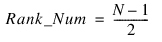
Rank Filtering
The rank filter is a nonlinear filter that can be used for removal of impulse noise. Each pixel in the result is computed as the rank of the filter window of N elements. The rank is defined as the value of the pixel in the Rank Number position when all pixels in the filtering window are arranged in ascending order. The rank filter degenerates to the Median filter when
Convolution
Convolution is a general process that can be used in smoothing, image processing, shifting, edge detection, and other filtering functions. Therefore, it is often used in conjunction with other functions, such as smoothing and shifting.
The Convolution Kernel parameter is an array whose dimensions describe the size of the neighborhood surrounding the value in the image that is analyzed. The Convolution Kernel also includes values that give a weighting to each point in its array. These weightings determine the average that is the value in the output array.
In many signal and image processing applications, it is useful to center a symmetric kernel over the data, to align the result with the original array. The Spot and Mirror options control the alignment of the Convolution Kernel with the input image and the ordering of the kernel elements.
Inverse Principle Components Transform (IPCT)
The inverse principle components transform (IPCT) differs from most inverse transforms in that the transformation matrix is not generic. The inverse transform can’t be performed without the transformation matrix, specified in the Transform Matrix portion of the dialog box. The Transform Matrix is generated with the PCT dialog box using the Transform option. The returned matrix is used in the Transform Matrix field of the IPCT dialog box.
Principle Components Transform
The principle components transform (also known as the Hotelling Transform, or the Karhunen-Loeve Transform) is commonly used in remote sensing applications. It de-correlates the input images, and the result contains the de-correlated images arranged according to the sample variance; that is, the image with the largest sample variance is first, and so on to the image with the smallest sample variance.
The principle components transform is computed by building a sample matrix, X, from the input image array. Each sample of X is a vector comprised of the corresponding pixels in each image of the array. The transformation matrix specified using the output array is then computed from the eigenvectors of the correlation matrix of X.
Lee Filter
The Lee Filter performs image smoothing by applying the Lee Filter algorithm. This algorithm assumes that the sample mean and variance of a value is equal to the local mean and variance of all values within a fixed range surrounding it. Lee Filter smooths additive noise by generating statistics in a local neighborhood and comparing them to the expected values.
Since Lee Filter is not very computationally expensive, it can be used for near real-time image processing.
For details on the Lee Filter, see the article by Jong-Sen Lee, “Digital Image Enhancement and Noise Filtering by Use of Local Statistics,” IEEE Transactions on Pattern Analysis and Machine Intelligence, Volume PAMI-2, Number 2, pages 165-168, March 1980.
Erosion
If the input image is not of the byte type, PV-WAVE makes a temporary byte copy of the image before using it for the processing.
The X Origin and Y Origin options specify the row and column coordinates of the structuring element’s origin. If omitted, the origin is set to the center, ([Nx / 2], [Ny / 2]), where Nx and Ny are the dimensions of the structuring element array. However, the origin need not be within the structuring element.
Nonzero elements of the structuring element determine the shape of the structuring element (neighborhood).
If the Structuring Element Values option is not specified, all elements of the structuring element are 0, yielding the neighborhood minimum operator. In addition the image is considered to be a binary image with all nonzero pixels considered as 1.
If you select Gray Scale Erosion, each pixel of the result is the minimum of the difference of the corresponding elements of the Structuring Element Values overlaid with the image.
Dilation
If the input image is not of the byte type, PV‑WAVE makes a temporary byte copy of the image before using it for the processing.
The X Origin and Y Origin options specify the row and column coordinates of the structuring element’s origin. If omitted, the origin is set to the center, ([Nx / 2], [Ny / 2]), where Nx and Ny are the dimensions of the structuring element array. However, the origin need not be within the structuring element.
Nonzero elements of the structuring element determine the shape of the structuring element (neighborhood).
If the Structuring Element Values option is not specified, all elements of the structuring element are 0, yielding the neighborhood minimum operator. In addition the image is considered to be a binary image with all nonzero pixels considered as 1.
If you select Gray Scale Erosion, each pixel of the result is the minimum of the difference of the corresponding elements of the Structuring Element Values overlaid with the image.
Interpolation
The Scale Dialog lets you shrink or expand the number of elements in the image by interpolating values at intervals where there might not have been values before. The resulting image is of the same data type as the input image.
Nearest Neighbor Method—Each output pixel is mapped to the input image and the nearest pixel is used for the result. The nearest neighbor interpolation method is not linear, because new values that are needed are merely set equal to the nearest existing value of the image. With high magnifications of regular structure, objectionable sawtooth edges result.
Bilinear interpolation—This method avoids sawtooth effect by determining the value of each output pixel by interpolating from the four neighbors of actual location in the input image. This method requires more computation time.
Image Shifting
The Shift Dialog Box is used to perform a circular shift upon the elements of an image.
“Circular” means that values that are pushed off the beginning or end of the array by the shift operation are automatically inserted back onto the opposite end of the array. No values in the array are lost.
The contents of entire rows and/or columns are shifted to the rows above or below, or to the columns to the right or left, depending on the number of rows and columns specified in the X Shift and Y Shift text fields respectively.
Positive numbers for the X Shift and Y Shift shift rows in an up direction (or columns to the right), while negative numbers shift rows in a down direction (or columns to the left).
The resulting image has the same dimension and data type as the input image.
Sample Usage
Typical uses of the Shift function include:

To force the elements of one array to align with the elements of another array.
To force the elements of one array to be misaligned with the elements of another array (some statistical analysis techniques require this).
To line up (or
register) the edges of an image to match those of another image. This can be used to compensate for an image that was initially digitized out of alignment with respect to the edges of another image.
To shift the beginning and ending point of a color table in an image.
Sobel Edge Enhancement
Sobel is commonly used to obtain an image that contains only the edges (rapid transitions between light and dark, or from one color to another) that were present in the original image. Sobel can help enhance features and transitions between areas in an image (for example, a machine part photographed against a white background).
With this information, it is possible to identify and compare features or items in an image with those in another image, usually for verification or detection purposes. Sobel and other edge-detection algorithms are used extensively for image processing and preprocessing for pattern recognition.
The image returned by Sobel contains the edges present in the original image, with the brightest edges representing a rapid transition (well-defined features), and darker edges representing smoother transitions (blurred or blended features).
An original image can also be somewhat sharpened by adding or averaging the edge-detected image with the original image.
Roberts Edge Enhancement
The Roberts function performs edge sharpening and isolation on the original image. It returns an approximation to the Roberts edge enhancement operator for images. This approximation is:
GA(j, k) = | Fj, k – Fj + 1, k + 1 | + | Fj, k + 1 – Fj + 1, k |
The resulting image returned by Roberts has the same dimensions as the input image.
note | Because the result image is saved in integer format, large original data values will cause overflow. Overflow occurs when the absolute value of the result is larger than 32,767. To avoid overflow, deselect the Clipping. |
Graylevel Run Length
Graylevel run length (GLRL) is used for
texture analysis of an image.
GLRL returns a 2D long array, result(m, n), where m is the graylevel minus the number of graylevels considered and n is the run length, ranging from 0 to N – 1 for an x-by-y image.
Run Length Angle = 45, or 135 degrees, N = (x2 + y2)1/2
Run Length Angle = 0, N = x
Run Length Angle = 90, N = y
The value at result(n, m) is the number of m-length runs at graylevel n + Minimum Value Considered.
Histogram Uses
Histograms are useful in a variety of applications, and can often provide signs as to what type of image processing should be performed. For example, photos sent back via satellite from outer space are usually accompanied by histograms. If the histogram for a photo contains a large spike, and the rest of the histogram is generally flat, this typically indicates that a histogram equalizing operation (such as the HIST_EQUAL function) is needed. Such an operation would spread out the pixels more evenly, thereby improving contrast and bringing out greater detail in the image.
Histograms can also be used to provide clues about images. For example, running a histogram on a series of identical photos taken at different times of the day may show the histogram peak shifting to the right—an indication that the average brightness is higher in that photo, and therefore more likely to be have been taken at a sunnier part of the day.
You can use histograms to compare two images of the same scene more fairly. By shifting the histogram of one scene so that it is aligned with that of the other scene, you can equalize the level of brightness in both images.
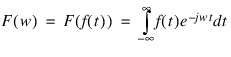
FFT Function
The Fourier transform of a scaled-time function is defined by:
where w relates to the frequency domain, and t relates to the time (space) domain.
Image Transforms
There are numerous transforms that can be applied to any image. The two most common transforms are the fast Fourier transform (FFT) and its inverse. The FFT converts an image from the spatial domain to the spatial frequency domain. Many other transforms exist, however, and are useful for various applications.
The Discrete Cosine Transform is also used in image compression. The Hough transform is useful in contour linking and identification of geometric shapes and lines in an image. This transform maps data from a cartesian coordinate space into a polar parameter space. The Slant transform uses sawtooth waveforms as a basis set and reveals connectivity.
The Principal Components Transform (PCT), also referred to as the Hotelling Transform or the Karhunen-Loeve Transform, is useful for image compression and de-correlation. This transform is widely used in remote sensing. The PCT is applied to the covariance matrix of the different spectral bands of a remote sensing image. Its output is an image that has a minimum amount of correlation. This maximum variance image combines most of the information present in the total spectral bands of the original image.
Smoothing
The Smooth dialog box is used to selectively average the elements in an array within a moving window of a given width. The result generally smooths out spikes or rapid transitions in the data, and fills in valleys and dips. This is usually called a boxcar average.
The window is a 2D region that traverses the input array, element by element, until it reaches the end. As the window moves across the array, all values within the window are averaged. The average value is then placed at the center of the window in the output array, while the original array is kept intact.
The smoothing window moves through the image from upper left to lower right.
The window may be any size as long as it is smaller than the array itself. Windows of 9, 25, 49, and 81 elements are typical. The value of Width does not appreciably affect the running time of the smoothing function.
Sample Usage
Typical uses for the Smooth function include:
To remove ripples, spikes, or high frequency noise from an image.
To blur an image such that only the general trends in the data can be seen (and are thereby highlighted).
To
isolate the lower spatial frequency components in an image. By subtracting a blurred image from the original image, only the higher spatial frequency components are left. (This is sometimes referred to as unsharp masking.)
To soften sharp transitions from one color to another in a color table. This helps reduce the banding or contouring artifact evident in color tables with rapid color changes.
Median Filtering
Median smoothing replaces each point with the median of the 2D neighborhood of the given width. It is similar to smoothing with a boxcar or average filter, but does not blur edges larger than the neighborhood. In addition, median filtering is effective in removing “salt and pepper” noise (isolated high or low values).
The scalar median is simply the middle value, which should not be confused with the average value (e.g., the median of [1, 10, 4] is 4, while the average is 5).
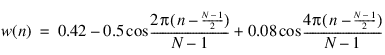
Window Domain Equations
A listing of the applicable time domain equations is given below, where (w(n), 0 < n < N – 1) for each of the windows.
Blackman window:
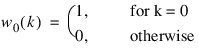
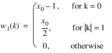
Chebyshev window:
for N = 0:
for N = 1:
for N > 1:
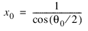
where:
and θ0 is the Windowing input parameter a.
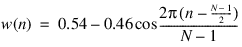
Hamming window:
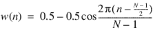
Hanning window:
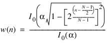
Kaiser window:
where I0(x) is the zeroth order Bessel function of the first kind, and α is the Windowing input parameter a.
Rectangular (or boxcar) window:
w(n) = 1, for all n.
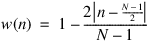
Triangular window:
for all n.
Graylevel Co-Occurrence Probability Matrix (GLCM)
Each element (a, b) of the graylevel co-occurrence matrix is the joint probability that graylevel b is at a distance specified by X Offset, and Y Offset from graylevel a. Performing statistics on the graylevel co-occurrence probability matrix (GLCM) provides quantitative information about image texture.
Sweet Spot
Defines the pixel location in the result array. The “sweet spot” is usually defined as the filter window center.
Rank Number
The rank number is used by a rank filter to process an image. The rank is defined as the value of the pixel in the rank number position when all the pixels in the filtering window are arranged in ascending order.
If the rank number equals the number of elements in the filtering window minus one or two, the rank filter degenerates to a median filter.
Blending
The current image and selected image (the operand) are blended using the a and b scale factors to produce an image that is the linear combination of the image and operand. Blending is sometimes used to produce a double exposure effect (e.g. fading one image out and another image in), or to combine segmented images into a single image for further analysis.
Filtering Window
Nonlinear filters, linear filters, spatial domain filters, and frequency domain filters use a filtering window.
Nonlinear filters operate by passing a small window over an image and computing an output image pixel based on a given nonlinear function of the input image pixels under that window. Typical window sizes are 3-by-3, 5-by-5 or 7-by-7 pixels-squared. Nonlinear filters are used for removal of so-called salt-and-pepper noise and Gaussian noise, as well as edge detection in an image.
Linear filters are defined by a filter kernel, which is itself just a small image. Filter kernels, also called windows, are usually 3-by-3, 5-by-5, or 7-by-7 pixels, which contain values that mathematically define the characteristics of the linear transform.
Filtering in the spatial domain is performed by the convolution between the image and a filter kernel. Convolution involves passing the filter kernel over the entire input image. Pixel values in the output image are defined at the corresponding location in the input image under the center pixel in the filter kernel. Output values for the edges of the image are ambiguous because part of the kernel hangs off the image edge. Typical methods for dealing with undefined output pixels is to simply copy the edge pixels from the input image directly to the output image or to extend the boundary of the input image by the size of the filter kernel before convolution.
Spatial frequency filters are most often used for image restoration and enhancement. Restoration algorithms remove degradation or noise that has corrupted the image. The Wiener filter and any circularly symmetric filters are good examples of this filtering technique.
Filtering in the frequency domain is performed by multiplying the frequency-domain image with a frequency-domain filter. The product of the image and the filter is then transformed back into the spatial domain by performing an inverse FFT. This technique of using the spatial domain is often used for filters with large kernels.
Range Filtering
The range filter is a nonlinear filter that can be used for edge detection.
Each pixel in the result is computed as the range (the maximum minus the minimum) of the wxdim*wydim pixels within the window defined by wxdim, wydim.
The pixel location in the result array is defined by the Sweet Spot values. In image processing, the window “sweet spot” is typically defined as the window center, or (wxdim*wydim-1)/2.
Mode Filtering
The mode filter is a nonlinear filter that can be used for noise removal.
Each pixel in the result is computed as the mode (the most frequent pixel value) of the wxdim*wydim pixels within the window defined by wxdim, wydim.
The pixel location in the result array is defined by the Sweet Spot values. In image processing, the window “sweet spot” is typically defined as the window center, or (wxdim*wydim-1)/2.
Geometric Mean Filtering
The geometric-mean filter is a nonlinear filter sometimes used for removing Gaussian distributed noise.
Each pixel in the result is computed as the product of the N pixels to the N –1 power within the filter window of N elements.
Maximum Filtering
The maximum filter is a nonlinear filter that can be used for removing outlying low or negative values from an image.
Each pixel in the result is computed as the maximum of the wxdim*wydim pixels within the window defined by wxdim, wydim.
The pixel location in the result array is defined by the Sweet Spot values. In image processing, the window “sweet spot” is typically defined as the window center, or (wxdim*wydim-1)/2.
Minimum Filtering
The minimum filter is a nonlinear filter that can be used for removing outlying high values from an image.
Each pixel in the result is computed as the minimum of the wxdim*wydim pixels within the window defined by wxdim, wydim.
The pixel location in the result array is defined by the Sweet Spot values. In image processing, the window “sweet spot” is typically defined as the window center, or (wxdim*wydim-1)/2.
Gaussian Noise Generation
The function generates pseudorandom numbers from a standard normal (Gaussian) distribution using an inverse CDF technique. In this method, a uniform (0, 1) random deviate is generated. Then, the inverse of the normal distribution function is evaluated at that point using the PV‑WAVE IMSL Statistics function NORMALCDF with keyword Inverse.
Uniform Noise Generation
Generates pseudorandom numbers from a uniform (0, 1) distribution using a multiplicative, congruential method.
Periodic Noise Generation
Periodic, or coherent, noise is composed of 2D sinusoidal functions. This is often seen in the form of electrical noise at 60 (or 50) Hz. In the spatial frequency domain, periodic noise corruption is easily seen as bright spot in the spectrum. A notch filter is generally useful in eliminated periodic noise from an image.
The formula for periodic noise is as follows:
n(i,j) = A sin(f0i + f1j)
Impulse Noise Generation
Impulse noise is often referred to as salt-and-pepper noise, and usually appears as bright and dark spots within an image. The High and Low keywords control the graylevel values for the salt (bright) and pepper (dark) noise, respectively. Salt and pepper noise are generated with equal probabilities, 0.5 each. In other words, one half of the noise is expected to be pepper noise and one half is expected to be salt noise. The probability parameter indicates the probability that a given pixel in the resulting image will be corrupted by noise. Typical values for probability are from 0.05 to 0.3.
Exponential Noise Generation
Generates pseudorandom numbers from a standard exponential distribution. The probability density function is f(x) = e–x, for x > 0. Uses an antithetic inverse CDF technique. In other words, a uniform random deviate U is generated, and the inverse of the exponential cumulative distribution function is evaluated at 1.0 – U to yield the exponential deviate.
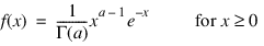
Gamma Noise Generation
The Gamma Noise Generation function generates pseudorandom numbers from a Gamma distribution with shape parameter A and output array dimensions. The probability density function follows:
Various computational algorithms are used depending on the value of the shape parameter A. For the special case of A = 0.5, squared and halved normal deviates are used; for the special case of A = 1.0, exponential deviates are generated. Otherwise, if A is less than 1.0, an acceptance-rejection method due to Ahrens, described in Ahrens and Dieter (1974), is used. If A is greater than 1.0, a 10-region rejection procedure developed by Schmeiser and Lal (1980) is used.
The Erlang distribution is a standard Gamma distribution with the shape parameter having a value equal to a positive integer; hence, the function generates pseudorandom deviates from an Erlang distribution with no modifications required.
Poisson Noise Generation
This function generates pseudorandom numbers from a Poisson distribution with positive mean Theta. The probability function (with θ = Theta) follows:
f(x) = (e–q θx)/x! , for x = 0, 1, 2, ...
If Theta is less than 15, the function uses an inverse CDF method; otherwise, the PTPE method of Schmeiser and Kachitvichyanukul (1981) is used. (See also Schmeiser, 1983.) The PTPE method uses a composition of four regions, a triangle, a parallelogram, and two negative exponentials. In each region except the triangle, acceptance/rejection is used. The execution time of the method is essentially insensitive to the mean of the Poisson.
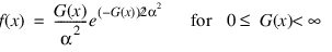
Rayleigh Noise Generation
Rayleigh noise is derived from uniform noise and is commonly seen in radar and velocity images. The probability density function for is:
Algebraic and Logical Point Operations
Algebraic, or mathematical
point operations used in image processing include addition, subtraction, multiplication, and, sometimes, a ratio of two images.
Logical operations such as AND, OR and exclusive OR can also be used to process images.
Use Algebraic operations to investigate differences or similarities between images. Image subtraction is a simple way to reveal image differences. Algebraic operations are also used for dynamic range scaling or shifting.
You must keep the pixel value range in mind when performing mathematical image operations because of the possibility of negative values in the result.
For example, when one image is subtracted from another, negative pixel values may result. Since the display color of a negative value is typically undefined, the resultant image values must be either clipped or shifted.
Another problem can occur when two images are multiplied together and the result contains values for which no corresponding color exists in the color map. These problems are called color map overflow and underflow.
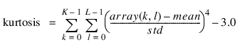
Kurtosis
Kurtosis is a useful measure for statistical texture analysis. The Kurtosis function computes the kurtosis of array(k, l) as:
where mean = AVG(array) and std = STDEV(array).
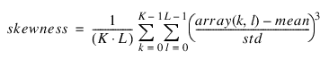
Skewness
Computes the skewness of array(k, l) as:
where mean = AVG(array) and std = STDEV(array).
The skewness is a useful measure for statistical texture analysis.
Standard Deviation and Variance
Mean, standard deviation and variance are basic statistical tools used in a variety of applications. They are computed as follows:
mean = TOTAL(array) / N_ELEMENTS(array)
stdev = SQRT(TOTAL((array – mean)^2) / (N_ELEMENTS(array) – 1))
variance = TOTAL((array – mean)^2) / (N_ELEMENTS(array) – 1)
Correlation
Correlation is sometimes used for template matching, and often used in conjunction with other methods such as thresholding to locate maxima in the correlation output. Correlation is computed in either the spatial or the spatial frequency domain. The spatial frequency domain computation is the default method for the Correlation Dialog Box. This method is used most often, and performs correlation as the multiplication of the FFT of the image with the conjugate of the FFT of the correlation template. The spatial domain computation, also called the direct method, performs correlation as the convolution operation without mirroring the filter kernel. The spatial domain computation is accomplished by selecting the Direct button in the Correlation dialog box.
K-Means Clustering
The K-Means Clustering dialog box computes a measurement vector for each individual pixel in the image. The measurements can be selected by using the Mean, Mode, Minimum, Maximum, Range, and Value options. If no statistical measures are selected through the use of these options, only the mean and mode statistics are used.
The K-Means function is a PV-WAVE:IMSL Statistics function used to identify clusters in image based on similar statistical features. The K-Means function computes Euclidean metric clusters for the measurement vectors. This begins with initial estimates of the mean values of the clusters determined from the Region Seed Points.
Growing Regions
Region growing is a segmentation method which uses the local pixel amplitude as the segmentation criteria. The Grow Region dialog performs image segmentation by pixel aggregation. Each region begins with a “seed” point as the initial region point. Neighboring pixels within a 3-by-3 area of each region point are then successively added to the region if the pixel value does not alter the region average by more than the value specified using the threshold option. When a new pixel is added to the region, the region average is updated to reflect all region members. The region growing process ends when no additional neighbors of the region pixels can be added to the region.
note | The Merge Region function should be used in place of Grow Region function when the region seed points are unknown. |
A pixel is added to a region if adding it does not alter the region average more than ± the threshold.
Region Splitting
Split Regions works best on images with separate square or rectangularly shaped regions. It is a recursive algorithm that subdivides the image into smaller and smaller units until either a homogeneous region is left or the maximum number of iterations has been reached.
note | Because the algorithm is recursive, Max Iterations should be kept reasonably small to avoid stack overflow problems. |
Region Merging
The algorithm for Region Merging analyzes each pixel in the image and attempts to add it to a region. The pixel may be added to a region, if its value does not change region average by more than the threshold.
The Region Merging function is useful for image segmentation and object identification and counting. This function can be used in place of, or in conjunction with, the Region Growing function. When the region seed points needed for the Region Growing function are unknown, the Region Merging function should be used instead.
When using Region Merging in conjunction with Region Growing, use the Region Growing function first, making sure that the Fill With Region Means option is set. Then, to reduce the number of regions grown, apply Region Merging with an appropriate threshold value.
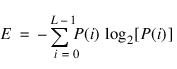
Entropy
Entropy is computed from the normalized image histogram P, where P is the histogram divided by its total as:
Top Hat
The morphological top-hat transform is used to identify small pixel clusters and edges. The peak detection top-hat operator is defined as the original image minus the opened image. The valley detection top-hat operator is defined as the closed image minus the original image.
Morphological Outlining
The morphological outline operator is defined as the difference between either the dilated or eroded image and itself. These operations are defined for byte data type images only. Outlining produces an output image in which all pixels are the background gray-level value except those pixels that lie on an object’s boundary. The thickness of the boundary is determined by the dimensions of the structuring element.
Hit or Miss Transform
The morphological hit-or-miss transform is useful for object and character recognition, because it can be used to identify features of a binary object. The hit-or-miss operator is defined as the intersection between the eroded image (eroded using the Hit Struct. Element) with the complement-eroded image (using the Miss Struct. Element parameter). Optimum results are obtained when Hit Struct. Element and Miss Struct. Element are disjoint. In other words, nonzero values of Hit Struct. Element are zero in Miss Struct. Element, and vice-versa.
Power Spectrum
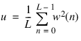
Spectrum computes one of several different power spectrum estimates P(f) depending on the input parameters. Specific estimates available include the periodogram, the modified periodogram, Bartlett’s method, and Welch’s method. In all cases uniform samples of the power spectrum are returned.
The equations shown below are for the case of a 1D signal, x, with a window length, L. (The derivation of the 2D equations is not shown here, but is found in most Image Processing references.)
The frequency sample values are:
fk = k/L , k = 0, 1, ..., M for real data.
where M = [(L + 2)/2] for L even and M = [(L + 1)/2] for L odd for real data.
For complex data, M = L.
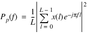
The periodogram is defined as
where the frequency variable f is normalized to the Nyquist frequency of 1.0. To obtain uniform samples of the periodogram using Spectrum, set length equal to the length of the data x, and set the window type to rectangular.
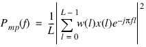
The modified periodogram is defined as:
where w(l) is a data window sequence. To obtain uniform samples of the modified periodogram using Spectrum, set length equal to the length of the data x and set the window type to any of the windows on the Window Type option menu.
Bartlett’s method breaks the data into non-overlapping data segments represented as
xi(n) = x(n + iL) n = 0, 1, ... , L – 1 i = 0, 1, ... , I – 1.
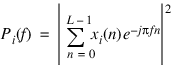
A periodogram:
is computed for each data segment and averaged to obtain the Bartlett estimate:
To obtain uniform samples of Bartlett’s estimate using Spectrum, set length to be less than the data length, set Overlap Fraction to 0 and set Window to rectangular.
The Welch method breaks the data into length L overlapping data segments represented as (n + iL).
xi(n) = x(n + iQ) n = 0, 1, ... , L – 1 i = 0, 1, ... , I – 1
where Q = (L – Overlap Fraction).
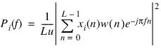
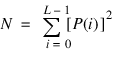
A modified periodogram is then computed for each data segment given by:
where:
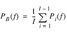
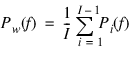
The Welch power spectrum estimate is the average of the modified periodogram of each data segment, given by:
To obtain uniform samples of the Welch estimate using Spectrum, set length less than the data length, set Overlap Fraction to a nonzero value and set Window to any of the available windows.
note | In estimating the power spectrum it is assumed that the input signal is stationary (i.e., the frequency content does not change with time). If the signal is non-stationary, the Wavelet dialog box can often provide better results than Spectrum. |
Canny Edge Detection
The Canny edge operator finds the local maxima in the gradient of the Gaussian-smoothed image. This is accomplished by applying a separable Gaussian gradient filter to the image, and then determining local maxima from each 3-by-3 neighborhood of the gradient magnitude image. These maxima are returned in the output image, with all non-maximal pixels set to 0.
Notch Filter
The Notch function produces a circularly symmetric, spatial frequency domain, ideal notch filter which can be applied to a frequency domain image. Notch filters are useful for removing narrow frequency ranges from images. Notch filtering is commonly used to remove periodic (coherent) noise.
Energy
Energy is computed from the normalized image histogram P, where P is the histogram divided by its total as:
Threshold Logic
To threshold an image, x, such that values between but not including 30 and 55 are set to 190 and all other values in x are 10, do the following:
Set
A to 30.
Set
B to 55.
Change
Set True to 190.
Change
Set False to 10.
Select the
Binary button.
Select A Logic:
NE.
Select B Logic:
NE.
This is conceptually the same as the following logic statement:
If 30 < x (i, j) < 55, then x (i, j) = 190, else x (i, j) = 10,
where 0 ≤ i < N and 0 ≤ j < M for all x (N, M).
Wavelet Transforms
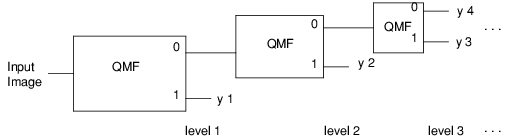
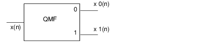
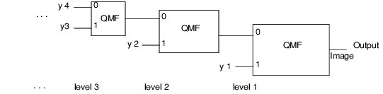
Computing the wavelet transform of an image using a compactly supported orthonormal wavelet is equivalent to applying the quadrature mirror filter-bank structure to the image as shown in the following figure.
The details of how and why the structure shown in the figure is connected to a compactly supported orthonormal wavelet are found in Akansu and Haddad, 1992; Daubechies, 1988, and 1992; Rioul and Vetterli, 1991; and Vaidyanathan, 1993.
The input and output sequences of each block in the figure represent the inputs and output of the forward part of the quadrature mirror filtering technique. The specific input-output relation between each block and the quadrature mirror filter is shown in the following figure.
The Wavelet dialog box requires a quadrature mirror filter to be supplied. Such a filter is obtained by using the IPQMFDESIGN function.
The Stages option specifies the number of levels of the wavelet transform structure to compute.
The backwards wavelet transform is computed using the filter bank structure shown in the following figure.
Filter Objects
For a spatial filter, the filter object has three strings containing the key names of elements of the associative array:
'kernel'—A 2D array of the filter spatial values.
'domain'—A string set to 'SPATIAL'.
'scale'—The scale factor.
For a spectral filter, the filter object has ten strings containing the key names of elements of the associative array:
'kernel'—A 2D array of the filter spectral values.
'domain'—A string set to 'SPECTRAL'.
'cutoff'—A one-element array (for highpass and lowpass filters), or a two-element array (for bandpass and bandstop filters) containing the filter cutoff frequency, or frequencies.
'pass'—A string indicating the filter type: 'low', 'high', 'stop', 'band', or 'notch'.
'dc_offset'—A float value containing the filter DC offset.
'co_frac'—A float value containing the fraction of the maximum filter value at the cutoff frequency.
'maximum'—A float value containing the maximum filter amplitude.
'type'—A string indicating the filter type: 'ideal', or 'Butterworth'.
'xloc'—(For notch filters only.) The x-location of the filter center.
'yloc'—(For notch filters only.) The y-location of the filter center.
'center'—If set, the filter center is at the center of the array.
'order'—(For Butterworth filters only.) A floating point value indicating the filter order.
Version 2017.0
Copyright © 2017, Rogue Wave Software, Inc. All Rights Reserved.