NONLINPROG Function (PV-WAVE Extreme Advantage)
Solves a general nonlinear programming problem using the successive quadratic programming (QP) algorithm.
Usage
result = NONLINPROG(f, m, n)
Input Parameters
f—A scalar string specifying a user-supplied procedure to evaluate the function at a given point. Procedure f has the following parameters:
 m
m—The total number of constraints.
meq—The number of equality constraints.
x—A one-dimensional array at which point the function is evaluated.
active—A one-dimensional array with
mmax components indicating the active constraints where
mmax is the maximum of (1,
m).
f—The computed function value at the point
x. (Output)
g—A one-dimensional array with
mmax components containing the values of the constraints at point
x, where
mmax is the maximum (1,
m). (Output)
m—The total number of constraints.
n—The number of variables.
Returned Value
result—The solution of the nonlinear programming problem.
Keywords
Double—If present and nonzero, double precision is used.
Err_Rel—The final accuracy. (Default: Err_Rel = ε1/2, where ε is the machine precision)
Grad—A scalar string specifying a user-supplied procedure to evaluate the gradients at a given point. The procedure specified by Grad has the following parameters:
mmax—The maximum of (1,
m).
m—The total number of constraints.
meq—The number of equality constraints.
x—The array at which point the function is evaluated.
active—An array with
mmax components indicating the active constraints.
f—The computed function value at the point
x.
g—An array with
mmax components containing the values of the constraints at point
x.
df—An array with
n components containing the values of the gradient of the objective function. (Output)
dg—An array of size
n-by-
mmax containing the values of the gradients for the active constraints. (Output)
Ibtype—A scalar indicating the types of bounds on the variables as shown in the following list.
0—User supplies all the bounds.
1—All variables are nonnegative.
2—All variables are non-positive.
3—User supplies only the bounds on first variable; all other variables have the same bounds.
Default: no bounds are enforced
Itmax—The maximum number of iterations allowed. (Default: Itmax = 200)
Meq—The number of equality constraints. (Default: Meg = m)
Obj—The name of a variable into which a scalar containing the value of the objective function at the computed solution is stored.
XGuess—An array with n components containing an initial guess of the computed solution. (Default: XGuess(*) = 0)
Xlb—A named variable, containing a one-dimensional array with n components, containing the lower bounds on the variables. (Input, if Ibtype = 0; Output, if Ibtype = 1 or 2; Input/Output, if Ibtype = 3). If there is no lower bound on a variable, the corresponding Xlb value should be set to –106 . (Default: no lower bounds are enforced on the variables)
XScale—Array with n components containing the reciprocal magnitude of each variable. Keyword XScale is used to choose the finite-difference step size, h. The i-th component of h is computed as ε1/2*max(|xi|, 1/si) *sign(xi), where ε is the machine precision, s = XScale, and sign(xi) = 1 if xi ≥ 0; otherwise, sign(xi) = –1. (Default: XScale(*) = 1)
Xub—A named variable, containing a one-dimensional array with n components, containing the upper bounds on the variables. (Input, if Ibtype = 0; Output, if Ibtype = 1 or 2; Input/Output, if Ibtype = 3). If there is no upper bound on a variable, the corresponding Xub value should be set to 106. (Default: no upper bounds are enforced on the variables)
Discussion
NONLINPROG is based on the subroutine NLPQL developed by Schittkowski (1986), and uses a successive quadratic programming method to solve the general nonlinear programming problem. The problem is stated as follows:
subject to:
gj(x) = 0 , for j = 0, ..., me –1
gj(x) ≥ 0 , for j = me, ..., m – 1
(xl ≤ x ≤ xu)
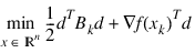
where all problem functions are assumed to be continuously differentiable. The method, based on the iterative formulation and solution of quadratic programming (QP) subproblems, obtains these subproblems by using a quadratic approximation of the Lagrangian and by linearizing the constraints. That is:
subject to:
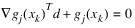
, for
j = 0, ...,
me –1
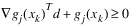
, for
j =
me, ...,
m –1
xl – xk ≤ d ≤ xu – xk
where Bk is a positive definite approximation of the Hessian and xk is the current iterate. Let dk be the solution of the subproblem. A line search is used to find a new point xk + 1:
xk + 1 = xk + λdk λ ∈ (0, 1]
such that a “merit function” has a lower function value at the new point. Here, the augmented Lagrange function (Schittkowski 1986) is used as the merit function.
When optimality is not achieved, Bk is updated according to the modified BFGS formula (Powell 1978). Note that this algorithm may generate infeasible points during the solution process. Therefore, if feasibility must be maintained for intermediate points, this function may not be suitable. For more theoretical and practical details, see Stoer (1985), Schittkowski (1983, 1986), and Gill et al. (1985).
For more details about the algorithms used by NONLINPROG, refer to the description of NONLINPROG in the PV‑WAVE IMSL Mathematics Reference.
Example
The problem:
min F(x) = (x1 – 2)2 + (x2 – 1)2
subject to:
g1(x) = x1 – 2x2 + 1 = 0
g2(x) = –x12/4 – x22 + 1 ≥ 0
is solved.
.RUN
; Define the procedure to evaluate the function at a given point.
PRO nlpex, m, meq, x, active, f, g
tmp1 = x(0) - 2.
tmp2 = x(1) - 1.
f = tmp1^2 + tmp2^2
g = FLTARR(2)
IF active(0) THEN g(0) = x(0) - 2. * x(1) + 1.
IF active(1) THEN g(1) = -(x(0)^2)/4. - x(1)^2 + 1.
END
% Compiled module: F.
; Compute the solution.
x = NONLINPROG('nlpex', 2, 2, Meq = 1)PM, x, Title = 'Solution:'
See Also
In the PV‑WAVE IMSL Mathematics Reference:
NONLINPROG
For Additional Information
Gill, Murray, Saunders and Wright, 1985. Powell, 1978.
Schittkowski, 1983, 1986. Stoer, 1985.
Version 2017.0
Copyright © 2017, Rogue Wave Software, Inc. All Rights Reserved.