NOISE_GEN Function (PV-WAVE Extreme Advantage)

Covariances—A 2D, square variance-covariance matrix defined for the Mvar_Normal distribution. The 2D result is of size n-by-N_ELEMENTS(Covariances(*, 0)).

note	Both the Covariances and Mvar_Normal keywords must be specified to return numbers from a multivariate normal distribution.

Double—If present and nonzero, double precision is used.

Exponential—If present and nonzero, uses the exponential distribution.

F1, ..., F8—(Used with the Periodic keyword.) The frequency for dimension i (i = 1, ..., 8) used for the periodic noise distribution.

Gamma—If present and nonzero, uses the gamma distribution.

High—The desired maximum of the returned values.

Impulse—If present and nonzero, uses the impulse distribution.

Low—The desired minimum of the returned values.

Mvar_Normal—If present and nonzero, uses the multivariate normal distribution.

note	Both the Mvar_Normal and Covariances keywords must be specified to return numbers from a multivariate normal distribution.

Normal—If present and nonzero, uses the normal distribution.

Periodic—If present and nonzero, uses the periodic distribution.

Pin—The first parameter of the beta distribution, a positive value.

Poisson—If present and nonzero, uses the Poisson distribution.

Prob—The noise probability for the impulse distribution.

Qin—The second parameter of the beta distribution, a positive value.

Rayleigh—If present and nonzero, uses the Rayleigh distribution.

S_Amp—A seed for the random number generator.

S_Index—A seed for the index random number generator.

Sine_Amp—The amplitude of sinusoidal (periodic) noise.

Theta—The mean value of the Poisson distribution, a positive value.

Type—A string indicating the desired data type of result. Valid strings include: 'byte', 'fix', 'float', or 'double'.

Uniform—If present and nonzero, uses the uniform distribution.

Var—The noise variance for the Rayleigh distribution.

The PV‑WAVE Image Processing Toolkit NOISE_GEN function is a wrapper for the noise generators which are already available in PV‑WAVE Advantage. Specifically, these include the RANDOM and RANDOMOPT routines in PV‑WAVE IMSL Statistics.

NOISE_GEN returns an array of noise with the probability distribution specified by the Normal, Poisson, Uniform, Impulse, Rayleigh, Exponential, Mvar_Normal, Beta, Gamma, and Periodic keywords. If NOISE_GEN is called without any keywords, then the returned array contains random numbers from a uniform (0, 1) distribution.

The default action of NOISE_GEN generates pseudo-random numbers from a uniform (0, 1) distribution using a multiplicative, congruent method. The form of the generator follows:

Each xi is then scaled into the unit interval (0, 1). The possible values for c in the generators are 16807, 397204094, and 950706376. The selection is made by using the RANDOMOPT procedure with the Gen_Option keyword. The choice of 16807 results in the fastest execution time. If no selection is made explicitly, the functions use the multiplier 16807.

The RANDOMOPT procedure called with the Set keyword is used to initialize the seed of the random-number generator.

You can select a shuffled version of these generators. In this scheme, a table is filled with the first 128 uniform (0,1) numbers resulting from the simple multiplicative congruent generator. Then, for each xi from the simple generator, the low-order bits of xi are used to select a random integer, j, from 1 to 128. The j-th entry in the table is then delivered as the random number, and xi, after being scaled into the unit interval, is inserted into the j-th position in the table.

The values returned are positive and less than 1.0. Some values returned may be smaller than the smallest relative spacing; however, it may be the case that some value, for example r(i), is such that 1.0 – r(i) = 1.0.

Deviates from the distribution with uniform density over the interval (a, b) can be obtained by scaling the output.

Calling RANDOM with keyword Normal generates pseudorandom numbers from a standard normal (Gaussian) distribution using an inverse CDF technique. In this method, a uniform (0, 1) random deviate is generated. Then, the inverse of the normal distribution function is evaluated at that point using the PV‑WAVE function NORMALCDF with keyword Inverse.

Deviates from the normal distribution with mean specific mean and standard deviation can be obtained by scaling the output from RANDOM.

Calling RANDOM with keyword Exponential generates pseudorandom numbers from a standard exponential distribution. The probability density function is f(x) = e–x, for x > 0. RANDOM uses an antithetic inverse CDF technique. In other words, a uniform random deviate U is generated, and the inverse of the exponential cumulative distribution function is evaluated at 1.0 – U to yield the exponential deviate.

Calling RANDOM with keywords Poisson and Theta generates pseudorandom numbers from a Poisson distribution with positive mean Theta. The probability function (with θ = Theta) follows:

If Theta is less than 15, RANDOM uses an inverse CDF method; otherwise, the PTPE method of Schmeiser and Kachitvichyanukul (1981) is used. (See also Schmeiser, 1983.) The PTPE method uses a composition of four regions, a triangle, a parallelogram, and two negative exponentials. In each region except the triangle, acceptance/rejection is used. The execution time of the method is essentially insensitive to the mean of the Poisson.

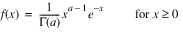
Calling RANDOM with keywords Gamma and A generates pseudorandom numbers from a Gamma distribution with shape parameter a = A and unit scale parameter. The probability density function follows:

Various computational algorithms are used depending on the value of the shape parameter a. For the special case of a = 0.5, squared and halved normal deviates are used; for the special case of a = 1.0, exponential deviates are generated. Otherwise, if a is less than 1.0, an acceptance-rejection method due to Ahrens, described in Ahrens and Dieter (1974), is used. If a is greater than 1.0, a 10-region rejection procedure developed by Schmeiser and Lal (1980) is used.

The Erlang distribution is a standard Gamma distribution with the shape parameter having a value equal to a positive integer; hence, RANDOM generates pseudorandom deviates from an Erlang distribution with no modifications required.

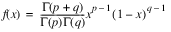
Calling RANDOM with keywords Beta, Pin, and Qin generates pseudorandom numbers from a beta distribution with parameters Pin and Qin, both of which must be positive. With p = Pin and q = Qin, the probability density function is:

where Γ( ⋅) is the Gamma function.

The algorithm used depends on the values of p and q. Except for the trivial cases of p = 1 or q = 1, in which the inverse CDF method is used, all the methods use acceptance/rejection. If p and q are both less than 1, the method of Jöhnk (1964) is used. If either p or q is less than 1 and the other is greater than 1, the method of Atkinson (1979) is used. If both p and q are greater than 1, algorithm BB of Cheng (1978), which requires very little setup time, is used if x is less than 4, and algorithm B4PE of Schmeiser and Babu (1980) is used if x is greater than or equal to 4.

note	Note that for p and q both greater than 1, calling RANDOM to generate random numbers from a beta distribution a loop getting less than four variates on each call yields the same set of deviates as executing one call and getting all the deviates at once.

The values returned are less than 1.0 and greater than ε, where ε is the smallest positive number such that 1.0 – ε < 1.0.

Calling RANDOM with keywords Mvar_Normal and Covariances generates pseudorandom numbers from a multivariate normal distribution with mean array consisting of all zeros and variance-covariance matrix defined using keyword Covariances. First, the Cholesky factor of the variance-covariance matrix is computed. Then, independent random normal deviates with mean zero and variance 1 are generated, and the matrix containing these deviates is post-multiplied by the Cholesky factor. Because the Cholesky factorization is performed in each invocation, it is best to generate as many random arrays as needed at once.

Deviates from a multivariate normal distribution with means other than zero can be generated by using RANDOM with keywords Mvar_Normal and Covariances, then adding the arrays of means to each row of the result.

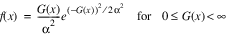
Calling NOISE_GEN with keywords Rayleigh and Var generates pseudorandom numbers from a Rayleigh distribution. With α = Var, the probability density function for Rayleigh noise is:

Calling NOISE_GEN with the Impulse and Prob keywords generates an array of impulse, or salt-and-pepper noise. Impulse noise appears as bright and dark spots within an image. The High and Low keywords control the graylevel values for the salt (bright) and pepper (dark) noise, respectively. Salt and pepper noise are generated with equal probabilities, 0.5 each. In other words, one half of the noise is expected to be pepper noise and one half is expected to be salt noise. The Prob keyword indicates the probability that a given pixel in the resulting image will be corrupted by noise. Typical values for Prob are from 0.05 to 0.3.

Calling NOISE_GEN with the Periodic and F1, ..., F8 keywords generates an array of periodic noise. Periodic, or coherent, noise is composed of 2D sinusoidal functions. This is often seen in the form of electrical noise at 60 (or 50) Hz. In the spatial frequency domain, periodic noise corruption is easily seen as bright spot in the spectrum. A notch filter is generally useful in eliminated periodic noise from an image.