DIST Function
Standard Library function that generates a square array in which each element equals the Euclidean distance from the nearest corner.
Usage
result = DIST(n, [m])
Input Parameters
n — The size of the resulting array.
m — If this parameter is supplied, the function generates a rectangular Euclidean distance array.
Returned Value
result — The resulting floating-point array.
Keywords
None.
Discussion
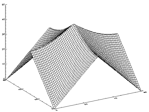
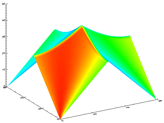
DIST generates a square array in which each element is proportional to its frequency. A three-dimensional plot of this function displays a surface where each quadrant is a curved quadrilateral forming a common cusp at the center.
The result of the DIST function is an n-by-n single-precision floating-point array, as defined by:
where:
F(x) = x if 0 ≤ x < n/2
or:
F(x) = n – 1 – x if x ≥ n/2
The DIST function is particularly useful for creating arrays that can be used for frequency domain filtering in image and signal processing applications.
note | DIST is an excellent choice when you need a two-dimensional array of any size for a fast test display. |
If the optional parameter m is supplied, the result is an n-by-m rectangular Euclidean distance array.
Example 1
Use the commands:
test_arr = DIST(60)
LOADCT, 18
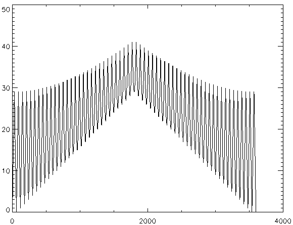
; Display data as a 2D plot
WINDOW, /Free
PLOT, test_arr, Background=WoColorConvert(255), Color=WoColorConvert(0)
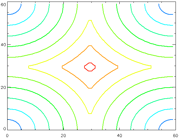
; Display data as a contour plot
WINDOW, /Free
CONTOUR, test_arr, Background=WoColorConvert(255), Color=WoColorConvert(0), $
Thick=2.0, Nlevels=9, $
C_Colors=WoColorConvert([50, 75, 100, 125, 150, 175, 200, 225, 250])
; Display data as a surface
WINDOW, /Free
SURFACE, test_arr, Linestyle=2, Background=WoColorConvert(255), $
Color=WoColorConvert(0)
; Display data as a shaded surface
WINDOW, /Free
SHADE_SURF, test_arr, Background=WoColorConvert(255), Color=WoColorConvert(0)
; Display data as an image
test_img = DIST(300)
WINDOW, Xsize=300, Ysize=300, /Free
TVSCL, test_img, 3
to create an array and display that array using multiple methods. The results are shown in the following images.
Example 2
This example shows how to use the DIST function to filter an image.
; Read the demo image.
mandril = BYTARR(512,512)
OPENR, unit, !Data_dir + 'mandril.img', /Get_lun
READU, unit, mandril
FREE_LUN, unit
; Use the DIST function to create a frequency image of the same
; size as the demo image.
d = DIST(512)
; Set n, the order (steepness) of Butterworth filter to use, and
; d0, the cutoff frequency.
n = 1.0
d0 = 10.0
; Create a Butterworth low-pass filter to be applied to the image.
filter = 1.0 / (1.0 + (d/d0)^(2.0 * n))
; Filter the image by transforming it to the frequency domain,
; multiplying by the filter, and then transforming back to the
; spatial domain.
filt_image = FFT(FFT(mandril, -1) * filter, 1)
; Display the original image.
WINDOW, XSize=1024, YSize=512, /Free, $
Title='Original Image (left) - Filtered Image (right)'
TVSCL, mandril, 2
; Display the resulting image.
TVSCL, filt_image, 1
See Also
For more information, see on frequency domain techniques, see the PV‑WAVE User’s Guide.
Version 2017.1
Copyright © 2019, Rogue Wave Software, Inc. All Rights Reserved.