LAGRANGE Function
Determines the coefficients for a Lagrange interpolating polynomial associated with a given set of abscissa points and function values.
Usage
lp = LAGRANGE(x, f)
Input Parameters
x—A vector containing the independent (abscissa) values of the data to be interpolated.
f—A vector containing data values to interpolate, where f(i) is the data associated with x(i).
Returned Value
lp—A vector containing coefficients of the Lagrange interpolating polynomial associated with x and f.
note | To evaluate the fitted Lagrange polynomial at a given point, apply the
POLY Function to lp. |
Keywords
None.
Discussion
None.
Example 1
; Here, we are trying to reproduce the function f(x) = x^2.
; f(1) = 1
; f(2) = 4
; f(3) = 9
PRINT, LAGRANGE([1, 2, 3], [1, 4, 9])
; PV-WAVE prints:
; 0.00000000 0.00000000 1.0000000
PRINT, POLY(5, LAGRANGE([1, 2, 3], [1, 4, 9]))
; PV-WAVE prints:
; 25.000000
Example 2
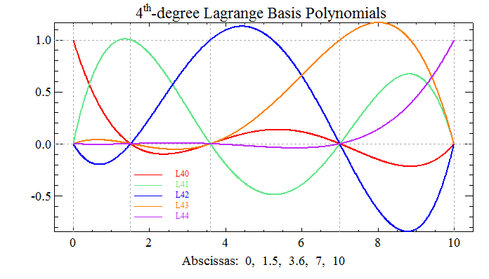
; Make up five abscissas to define five, 4th-degree,
; Lagrange basis polynomials on.
x = [0.0, 1.5, 3.6, 7, 10]
; Define the function values associated with each of the
; five Lagrange basis polynomials. By definition, the
; polynomial associated with the 0th abscissa will equal 1
; at x(0)=0, while the other four polynomials will equal 0.
; Likewise, the polynomial associated with the 1st abscissa
; will equal 1 at x(1)=1.5, while the other four polynomials
; will equal 0, etc.
y = [1, 0, 0, 0, 0]
L40 = LAGRANGE(x, y)
; L40 means the 4th-degree Lagrange basis polynomial
; associated with the 0th abscissa.
y = [0, 1, 0, 0, 0]
L41 = LAGRANGE(x, y)
y = [0, 0, 1, 0, 0]
L42 = LAGRANGE(x, y)
y = [0, 0, 0, 1, 0]
L43 = LAGRANGE(x, y)
y = [0, 0, 0, 0, 1]
L44 = LAGRANGE(x, y)
; Now evaluate the five Lagrange basis polynomials
; over the domain x=[0, 10].
domain = INTERPOL([0, 10], 1000)
P40 = POLY(domain, L40)
P41 = POLY(domain, L41)
P42 = POLY(domain, L42)
P43 = POLY(domain, L43)
P44 = POLY(domain, L44)
; Plot each of the basis polynomials.
!P.font = 0
TEK_COLOR
clrs = WoColorConvert(INDGEN(256))
WINDOW, /Free, Xsize=700, Ysize=400
minY = MIN([P40, P41, P42, P43, P44], Max=maxY)
PLOT, domain, P40, /Nodata, Xrange=[-0.5, 10.5], $
Yrange=[minY,maxY], Ystyle=1, Xstyle=1, $
Title='4!eth!N-degree Lagrange Basis Polynomials', $
Xtitle='Abscissas: 0, 1.5, 3.6, 7, 10', $
Color=clrs(0), Background=clrs(1)
OPLOT, !X.Crange, [0, 0], Linestyle=1, Color=clrs(15)
OPLOT, !X.Crange, [1, 1], Linestyle=1, Color=clrs(15)
FOR i=0L,4 DO OPLOT, [x(i), x(i)], !Y.Crange, $
Linestyle=1, Color=clrs(15)
line_clrs = clrs([2, 25, 4, 8, 30])
OPLOT, domain, P40, Thick=2, Color=line_clrs(0)
OPLOT, domain, P41, Thick=2, Color=line_clrs(1)
OPLOT, domain, P42, Thick=2, Color=line_clrs(2)
OPLOT, domain, P43, Thick=2, Color=line_clrs(3)
OPLOT, domain, P44, Thick=2, Color=line_clrs(4)
; Add a legend.
oldCharsize = !P.Charsize
!P.charsize = 0.75
labels = ['L40', 'L41', 'L42', 'L43', 'L44']
line_types = REPLICATE(!P.linestyle, 5)
psyms = REPLICATE(!P.psym, 5)
LEGEND, labels, line_clrs, line_types, psyms, 1.6, -0.3, 0.1
!P.charsize = oldCharsize
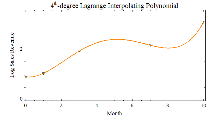
Example 3
; Make up some function data to go with the abscissa values.
sales_data = [0.918, 1.056, 1.906, 2.134, 3.029]
month = [0, 1, 3, 7, 10]
WINDOW, /Free, Xsize=700, Ysize=400
!P.font = 0
TEK_COLOR
clrs = WoColorConvert(INDGEN(256))
PLOT, month, sales_data, Psym=2, Xrange=[-0.1, 10.1], $
Yrange=[0, 3.5], Ystyle=1, Xstyle=1, $
Xtitle='Month', Ytitle='Log Sales Revenue', $
Title='4!eth!N-degree Lagrange Interpolating Polynomial', $
Color=clrs(0), Background=clrs(1)
; Fit the Lagrange interpolating polynomial to the data and plot it.
l_val = LAGRANGE(month, sales_data)
x_val = INTERPOL([0,10], 1000)
p_val = POLY(x_val, l_val)
OPLOT, x_val, p_val, Color=clrs(8), Thick=2
See Also
Version 2017.1
Copyright © 2019, Rogue Wave Software, Inc. All Rights Reserved.