Parameter Calculation Classes

Business Analysis Module User's Guide
Rogue Wave web site: Home Page | Main Documentation Page

5.5 Parameter Calculation Classes

The parameter calculation method used for models is determined by classes that derive from the abstract base class RWRegressionCalc. The parameter calculation method used by a particular regression object may be specified by providing an instance of a class derived from RWRegressionCalc to the regression object at construction time, or through the regression class member function setCalcMethod(). If you do not specify a calculation method at construction time, a default method is provided.

Encapsulating parameter calculations in a class yields two benefits:

Calculation methods can be changed at runtime. For example, if you choose a calculation method that is fast but fails on a particular set of data, you can switch to a slower, more robust method.
You can use your own calculation method by deriving a class from RWRegressionCalc and providing the calculation method.

Here is an example of how to switch calculation methods at runtime:

RWMathVec<double> observations;
RWGenMat<double> predictorMatrix;
.
.
.
// Construct a linear regression object using the default
// calculation method class RWLeastSqQRCalc.  This
// method is fast, but will fail if the regression matrix does
// not have full rank.

RWLinearRegression lr(  predictorMatrix, observations);
if ( lr.fail() )
{
  // Try the more robust, but slower QR with pivoting method:
  lr.setCalcMethod(RWLeastSqQRPvtCalc());
  if ( lr.fail() )
  {
    // Matrix must have a column of 0s or something. 
    // Deal with the error.
    cerr << "Parameter calculation failed for input data." << endl;
  }
  else
  {
    cout << "Parameters calculated using the QR with pivoting
             method: " << lr.parameters() << endl;
  }
}
else
{
  cout << "Parameters calculated using the QR method: " << lr.parameters() << endl;
}
.
.
.

All parameter calculation classes have a member function, called name(), which returns a string identifying the calculation method. In the convention used by the Business Analysis Module, name() returns the class static variable methodName. For example, if you want to know whether a particular logistic regression object uses the Levenberg-Marquardt calculation method, you would proceed as follows:

.
.
.
RWMathVec<double> observations;
RWGenMat<double> predictorMatrix;
.
.
.
RWLogisticRegression lr(predictorMatrix, observations);
.
.
.
// Check which calculation method is being used by the regression.
if ( lr.calcMethod().name() ==                         RWLogisticLevenbergMarquardt::methodName )
{
  cout << "using Levenberg-Marquardt calculation method" << endl;
}
else
{
  cout << "using something else" << endl;
}
.
.
.

5.5.1 Calculation Methods for Linear Regression

Given the linear regression model Y = βx + ε, finding the least squares solution is equivalent to solving the normal equations . Thus the solution for is given by:

The Business Analysis Module includes three classes for calculating multiple linear regression parameters: RWLeastSqQRCalc, RWLeastSqQRPvtCalc, and RWLeastSqSVDCalc. The following three sections provide a brief description of the method encapsulated by each class, and its pros and cons.

5.5.1.1 RWLeastSqQRCalc

Class RWLeastSqQRCalc encapsulates the QR method. This method begins by decomposing the regression matrix X into the product of an orthogonal matrix Q and an upper triangular matrix R. The QR representation is then substituted into the equation in Section 5.5.1 to obtain the solution .

Pros:

Good performance. Parameter values are recalculated very quickly when adding or removing predictor variables. Model selection performance is best with this calculation method.

Cons:

Calculation fails when the regression matrix X has less than full rank. (A matrix has less than full rank if the columns of X are linearly dependent.) Results may not be accurate if X is extremely ill-conditioned.

5.5.1.2 RWLeastSqQRPvtCalc

Class RWLeastSqQRPvtCalc uses essentially the same QR method described in Section 5.5.1.1, except that the QR decomposition is formed using pivoting.

Pros:

Calculation succeeds for regression matrices of less than full rank. However, calculations fail if the regression matrix contains a column of all 0s.

Cons:

Slower than the straight QR technique described in Section 5.5.1.1.

5.5.1.3 RWLeastSqSVDCalc

Class RWLeastSqSVDCalc employs singular value decomposition (SVD). The method solves the least squares problem by decomposing the regression matrix into the form , where P is an matrix consisting of p orthonormalized eigenvectors associated with the p largest eigenvalues of , Q is a orthogonal matrix consisting of the orthonormalized eigenvectors of , and Σ = diag(σ₁, σ₂, ... , σ_p) is a diagonal matrix of singular values of X. This singular value decomposition of X is used to solve the equation in Section 5.5.1.

Pros:

Works on matrices of less than full rank. Produces accurate results when X has full rank, but is highly ill-conditioned.

Cons:

Slower than the straight QR technique described in Section 5.5.1.1.

5.5.2 Calculation Methods for Logistic Regression

Unlike linear regression, where finding parameters involves solving a system of linear equations, parameter calculation for logistic regression requires the solution of a system of nonlinear equations. The equations become nonlinear because each prediction from the logistic regression model has its own estimated variance; the particular variance estimate influences the prediction, while the estimated prediction influences the estimated variance. The only way to find a solution to these nonlinear equations involves using an iterative, gradient-based algorithm.

For finding the parameters to a logistic regression model, the Business Analysis Module supplies two classes: RWLogisticIterLSQ and RWLogisticLevenbergMarquardt. The following sections provide a brief description of the method encapsulated by each class, along with its pros and cons.

5.5.2.1 RWLogisticIterLSQ

Class RWLogisticIterLSQ uses iterative least squares for finding logistic regression parameters. Some people also refer to this algorithm as the Newton-Raphson method. The algorithm starts with a set of parameters that corresponds to a linear fit of the data using the normal equations. Then the method repeatedly forms at iteration k by solving the linear equations:

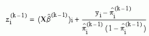
where X is the regression matrix, V^{(k – 1)} is the diagonal matrix of variance estimates at iteration k – 1, and z^{(k – 1)} is a vector of adjusted predictions at iteration k – 1. Element i of z^{(k – 1)} is defined as:

The algorithm stops iterating when the size of the change in parameter values falls below a small, predetermined value. The default value is macheps^(2/3), where macheps is the value of machine epsilon.

Pros:

Iterative least squares is one of the fastest algorithms for finding logistic regression parameters.

Cons:

If the initial parameter estimate is poor, the algorithm is not guaranteed to converge successfully, while a more sophisticated algorithm might converge.

5.5.2.2 RWLogisticLevenbergMarquardt

Class RWLogisticLevenbergMarquardt finds logistic regression parameters using a more sophisticated technique than iterative least squares. It implements what is known as the Levenberg-Marquardt method. The extra sophistication of this algorithm often causes a recovery from poor initial estimates for . The starting vector of parameters is the same as for iterative least squares, and at each iteration, the algorithm tries to take a step that is similar to the one taken by iterative least squares. However, it checks to make sure that the step improves the likelihood of the model producing the data. If the step does improve likelihood, the step is taken. If the step does not improve likelihood, the algorithm tries a modified step that falls closer to the gradient. This process of checking and trying a step even closer to the gradient repeats until a step is found that finally improves the likelihood. For further discussion of this and similar optimization algorithms, see Dennis & Schnabel, Numerical Methods for Unconstrained Optimization and Nonlinear Equations, Prentice-Hall, (1983).

Pros:

If the initial parameter estimate is poor, the algorithm often still converges to a set of finite-valued parameters, while iterative least squares may not.

Cons:

The algorithm is slower than iterative least squares.

5.5.3 Writing Your Own Parameter Calculation Class

You can incorporate your own parameter calculation methods into the Business Analysis Module by supplying your own parameter calculation class. Your class must be derived from the abstract base class RWRegressionCalc and must implement its five pure virtual functions:

virtual void 
calc(const RWGenMat<T>& r, const RWMathVec<S>& o) = 0;

Calculates the model parameters from the input regression matrix r and observation vector v.

virtual RWMathVec<T>
parameters() = 0;

Returns the calculated parameters.

virtual bool 
fail() const = 0;

Returns true if the most recent calculation failed. Otherwise, returns false.

virtual RWCString 
name() const = 0;

Returns name identifying the calculation method.

virtual RWRegressionCalc<T,S>* 
clone() = 0;

Returns a copy of self off the heap.

Here is an example of a calculation class for linear regression that uses the DoubleLeastSqCh class (replaced by class RWLeastSqCh<T>) found in the Linear Algebra Module of SourcePro Analysis:

class CholeskyLeastSquaresCalc : public RWRegressionCalc<double,double>
{
public:
static const char *methodName;

  // Constructors-----------------------------------------------
 CholeskyLeastSquaresCalc (){;}
 CholeskyLeastSquaresCalc ( const CholeskyLeastSquaresCalc & c )
   :parameters_(c.parameters_),fail_(c.fail_)
{
   // Make sure I have my own copy of the parameters.
   parameters_.deepenShallowCopy();
}

  //------------------------------------------------------------
  // Pure virtual functions inherited from RWRegressionCalc 
  // (see regcalc.h for function descriptions).
  //------------------------------------------------------------
  virtual void calc( const RWGenMat<double>& regressionMatrix, 
                     const RWMathVec<double>& observations)
  {
    DoubleLeastSqCh lsqch( regressionMatrix );
    fail_ = lsqch.fail();
    if ( !lsqch.fail() )
    {   
      parameters_.reference( lsqch.solve( observations ) ); 
    }
  }

  virtual RWRegressionCalc<double,double>* clone() const { 
           return new CholeskyLeastSquaresCalc ( *this ); }

  virtual RWMathVec<double> parameters()
  {
      if ( fail() ) // Clients should check fail status before 
                    // they call parameters().
      {
       RWTHROW( RWInternalErr("Parameters Failed.") );
        // Keeps some compilers happy.
        return parameters_;
      }
      else
     {
        return parameters_;
      }
  }

  virtual bool         fail() const { return fail_; }
  virtual RWCString    name() const { return methodName; }
  
// Assignment operator.
  RWLeastSqSVDCalc& operator=( const RWLeastSqSVDCalc& rhs )
  {
    parameters_.reference( rhs.parameters_ );
    parameters_.deepenShallowCopy();
    fail_ = rhs.fail_;
    return *this;
  }

private:
  RWMathVec<double> parameters_;
  bool              fail_;
};

The Rogue Wave name and logo, and SourcePro, are registered trademarks of Rogue Wave Software. All other trademarks are the property of their respective owners.
Provide feedback to Rogue Wave about its documentation.

Pros:	Good performance. Parameter values are recalculated very quickly when adding or removing predictor variables. Model selection performance is best with this calculation method.
Cons:	Calculation fails when the regression matrix X has less than full rank. (A matrix has less than full rank if the columns of X are linearly dependent.) Results may not be accurate if X is extremely ill-conditioned.

Pros:	Calculation succeeds for regression matrices of less than full rank. However, calculations fail if the regression matrix contains a column of all 0s.
Cons:	Slower than the straight QR technique described in Section 5.5.1.1.

Pros:	Works on matrices of less than full rank. Produces accurate results when X has full rank, but is highly ill-conditioned.
Cons:	Slower than the straight QR technique described in Section 5.5.1.1.

Pros:	Iterative least squares is one of the fastest algorithms for finding logistic regression parameters.
Cons:	If the initial parameter estimate is poor, the algorithm is not guaranteed to converge successfully, while a more sophisticated algorithm might converge.