3.2 Multiple Linear Regression
In the late 1880s, Francis Galton was studying the inheritance of physical characteristics. In particular, he wondered if he could predict a boy’s adult height based on the height of his father. Galton hypothesized that the taller the father, the taller the son would be. He plotted the heights of fathers and the heights of their sons for a number of father-son pairs, then tried to fit a straight line through the data. If we denote the son’s height by HS and the father’s height by HF, we can say that in mathematical terms, Galton wanted to determine constants β0 and β1 such that:
HS= β0 + β1HF
This is an example of a simple linear regression problem with a single predictor variable, HF. The parameter β0 is called the intercept parameter. In general, a regression problem may consist of several predictor variables. Thus the multiple linear regression problem may be stated as follows:
Let Y be a random variable that can be expressed in the form:
Y = β0 + β1x1 + ... + βp – 1 + ε
where x1, x2, ... , xp – 1 are known constants, and ε is a fluctuation error. The problem is to estimate the parameters βj. If the xj are varied and the n values Y1, Y2, ..., Yn of Y are observed, then we write:
Yi = β0 + β1xi1 + ... + βp – 1xi, p – 1 + εi (i = 1, 2, ..., n)
where x
ij is the
ith value of x
j. Writing these
n equations in matrix form we have:
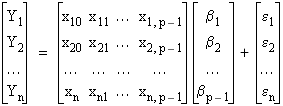
or:
Y = Xβ + ε
where x10 = x20 = ... = xn0 = 1
We call the

matrix
X the
regression matrix, each Y
i a
response variable,
Y the
response vector, and x
j the
predictor variable.
3.2.1 Parameter Calculation by Least Squares Minimization
The
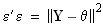
method of least squares consists of minimizing

with respect to
β. Setting
θ = X
β, we minimize:
subject to:

Let

be the least squares estimate of
β. The fitted regression

is denoted by:

The elements of
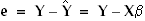
are called the
residuals. The value of:
is called the
residual sum of squares. The matrix:
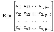
which is the regression matrix without the first column of 1s, is called the predictor data matrix.
3.2.2 Model Variance
The variance of the model is defined to be the variance of
ε. The statistic:

is an unbiased estimator of this variance.
3.2.3 Parameter Dispersion (Variance-Covariance) Matrix
The
dispersion matrix for the parameter estimates
is the matrix
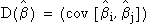
, where

is the covariance of

and

. The dispersion matrix is calculated according to the formula
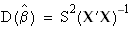
where S
2 is the estimated variance, as defined above, and
X and

are the regression matrix and its transpose, respectively.
3.2.4 Significance of the Model (Overall F Statistic)
The
overall F statistic is a statistic for testing the null hypothesis
β1 =
β2 = ... =
βp – 1 = 0. It is defined by the equation:
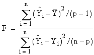
where

This statistic follows an F distribution with (p-1) and (n-p) degrees of freedom.
3.2.4.1 p-Value
The p-value is the probability of seeing the value of the F statistic for a given linear regression if the null hypothesis:
β0 = β1 = ... = βp – 1 = 0
is true.
3.2.4.2 Critical Value
The critical value of the F statistic for a specified significance level, α , is the value, v, of the F statistic such that if the F statistic calculated for the multiple linear regression is greater than v, we reject the hypothesis β1 = β2 = ... = βp – 1 = 0 at the significance level α.
3.2.5 Significance of Predictor Variables
Let
be the estimate for element
j of the parameter vector
β. The T statistic for the parameter estimate
is a statistic for testing the hypothesis that

It is calculated according to the formula:
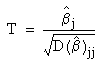
where

is the
jth diagonal element of the dispersion matrix. This statistic is assumed to follow a T distribution with
n –
p degrees of freedom.
3.2.5.1 p-Values
The
p-value for each parameter estimate
is the probability of seeing the value of the calculated parameter using the formula in
Section 3.2.5 if the hypothesis
βj = 0 is true.
3.2.5.2 Critical Values
The critical value of a parameter T statistic for a given level of significance
α is the value
vj, such that if the absolute value of the T statistic calculated for a given parameter
is greater than v
j, we reject the hypothesis
βj = 0 at the significance level
α.
3.2.6 Prediction Intervals
Suppose that we have calculated parameter estimates
for our linear regression problem. Suppose further that we have a vector of values,
x, for the predictor variables. We may obtain an
α level confidence interval for the value

, which is the value of the dependent of the observed variable predicted by our model, according to the formula:
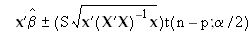
where t(n – p;α/2) is the value at α/2 of the cumulative distribution function for a T distribution, S is the estimated variance, and X is the regression matrix.