SIMPLESTAT Function (PV-WAVE Advantage)
Computes basic univariate statistics.
Usage
result = SIMPLESTAT(x)
Input Parameters
x—Data matrix. The data value for the ith observation of the jth variable should be in the matrix element (i, j).
Returned Value
result—A two-dimensional matrix containing some simple statistics for each variable
x. If
Median and
Median_And_Scale are not used as keywords, then element (
i,
j) of the returned matrix contains the
ith statistic of the
jth variable. Refer to
SIMPLESTAT Results for a list of results.
Input Keywords
Double—If present and nonzero, double precision is used.
Conf_Means—Scalar specifying the confidence level for a two-sided interval estimate of the means (assuming normality) in percent. The Conf_Means keyword must be between 0.0 and 100.0 and is often 90.0, 95.0, or 99.0. For a one-sided confidence interval with confidence level c, set Conf_Means = 100.0 – 2.0(100.0 – c) (at least 50 percent). Default: 95-percent confidence interval is computed
Conf_Variances—Confidence level for a two-sided interval estimate of the variances (assuming normality) in percent. The confidence intervals are symmetric in probability (rather than in length). For one-sided confidence interval with confidence level c, set Conf_Means = 100.0 – 2.0(100.0 – c) (at least 50 percent). Default: 95-percent confidence interval is computed.
Median_Only—If present and nonzero, medians are computed and stored in elements (14, *) of the returned matrix of simple statistics. The Median_Only and Median_And_Scale keywords cannot be used together.
Median_And_Scale—If present and nonzero, specified, the medians, the medians of the absolute deviations from the medians, and a simple robust estimate of scale are computed and stored in elements (14, *), (15, *), and (16, *) of the returned matrix of simple statistics. The Median_Only and Median_And_Scale keywords cannot be used together.
Elementwise—If present and nonzero, all nonmissing data for any variable is used in computing the statistics for that variable. Default: if an observation (row of x) is missing a value, the observation is excluded from computations for all variables. In either case, if weights and/or frequencies are specified and the value of the weight and/or frequency is missing, the observation is excluded from computations for all variables.
Frequencies—One-dimensional array containing the frequency for each observation. Default: each observation has a frequency of 1
Weights—One-dimensional array containing the weight for each observation. Default: each observation has a weight of 1
Discussion
Function SIMPLESTAT computes the sample mean, variance, minimum, maximum, and other basic statistics for the data in x. It also computes confidence intervals for the mean and variance (under the hypothesis that the sample is from a normal population).
Frequencies, fi’s, are interpreted as multiple occurrences of the other values in the observations. In other words, a row of x with a frequency variable having a value of 2 has the same effect as two rows with frequencies of 1. The total of the frequencies is used in computing all the statistics based on moments (mean, variance, skewness, and kurtosis). Weights, wi’s, are not viewed as replication factors. The sum of the weights is used only in computing the mean (the weighted mean is used in computing the central moments). Both weights and frequencies can be zero, but neither can be negative. In general, a zero frequency means that the row is to be eliminated from the analysis; no further processing or error checking is done on the row. A weight of zero results in the row being counted, and updates are made of the statistics.
The definitions of some of the statistics are given below in terms of a single variable x of which the ith datum is xi.
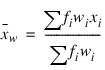
Mean
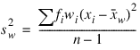
Variance
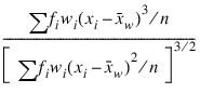
Skewness
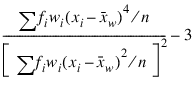
Excess or Kurtosis
Minimum
xmin = min(xi)
Maximum
xmax = max(xi)
Range
xmax – xmin
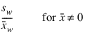
Coefficient of Variation
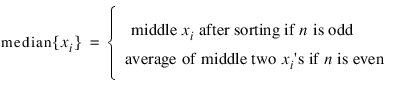
Median
Median Absolute Deviation
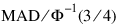
Simple Robust Estimate of Scale
where
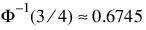
is the inverse of the standard normal distribution function evaluated at 3/4. This standardizes MAD in order to make the scale estimate consistent at the normal distribution for estimating the standard deviation (Huber 1981, pp. 107–108).
Example
This example uses data from Draper and Smith (1981). There are five variables and 13 observations.
x = STATDATA(5)
; Call SIMPLESTAT.
stats = SIMPLESTAT(x)
; Define the character strings that will be used as labels for the
; rows of the output.
labels = ['means', 'variances', 'std. dev', 'skewness', $
'kurtosis', 'minima', 'maxima', 'ranges', 'C.V.', 'counts', $
'lower mean', 'upper mean', 'lower var', 'upper var']
FOR i=0L, 13 DO PM, labels(i), stats(i, *), $
Format = '(a10, 5f9.3)'
Output the results:
means 7.462 48.154 11.769 30.000 95.423
variances 34.603 242.141 41.026 280.167 226.314
std. dev 5.882 15.561 6.405 16.738 15.044
skewness 0.688 -0.047 0.611 0.330 -0.195
kurtosis 0.075 -1.323 -1.079 -1.014 -1.342
minima 1.000 26.000 4.000 6.000 72.500
maxima 21.000 71.000 23.000 60.000 115.900
ranges 20.000 45.000 19.000 54.000 43.400
C.V. 0.788 0.323 0.544 0.558 0.158
counts 13.000 13.000 13.000 13.000 13.000
lower mean 3.907 38.750 7.899 19.885 86.332
upper mean 11.016 57.557 15.640 40.115 104.514
lower var 17.793 124.512 21.096 144.065 116.373
upper var 94.289 659.817 111.792 763.434 616.688
Version 2017.0
Copyright © 2017, Rogue Wave Software, Inc. All Rights Reserved.