NONLINREGRESS Function (PV-WAVE Advantage)
Fits a nonlinear regression model.
Usage
result = NONLINREGRESS(fcn, n_parameters, x, y)
Input Parameters
fcn—Scalar string specifying the name of a user-supplied function to evaluate the function that defines the nonlinear regression problem. Function fcn accepts the following input parameters and returns a scalar float:
 x
x—One-dimensional array containing the point at which point the function is evaluated.
theta—One-dimensional array containing the current values of the regression coefficients. Function
fcn returns a predicted value at the point
x. In the following,
f(
xi;
θ), or just
fi, denotes the value of this function at the point
xi, for a given value of
θ. (Both
xi and
θ are arrays.)
n_parameters—Number of parameters to be estimated.
x—Two-dimensional array containing the matrix of independent (explanatory) variables.
y—One-dimensional array of length N_ELEMENTS (x(*, 0)) containing the dependent (response) variable.
Returned Value
result—One-dimensional array of length n_parameters containing solution:
for the nonlinear regression coefficients.
Input Keywords
Double—If present and nonzero, double precision is used.
Theta_Guess—Array with n_parameters components containing an initial guess. Default: Theta_Guess(*) = 0
Jacobian—Scalar string specifying the name of a user-supplied function to compute the ith row of the Jacobian. This function accepts the following parameters:
X—One-dimensional array of length N_ELEMENTS (
x(0, *)) containing the data values corresponding to the
ith row.
Theta—One-dimensional array of length
n_parameters containing the regression coefficients for which the Jacobian is evaluated. The return value of this function is an array of length
n_parameters containing the computed
n_parameters row of the Jacobian for observation
i at
Theta. Note that each derivative
∂f(
xi)/
∂θj should be returned in element (
j – 1) of the returned array for
j = 1, 2, ...,
n parameters.
Theta_Scale—One-dimensional array of length n_parameters containing the scaling array for θ. Keyword Theta_Scale is used mainly in scaling the gradient and the distance between two points. See keywords Grad_Eps and Step_Eps for more details. Default: Theta_Scale(*) = 1
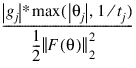
Grad_Eps—Scaled gradient tolerance. The jth component of the scaled gradient at θ is calculated as:
where
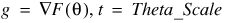
, and
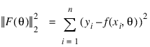
The value F(θ) is the vector of the residuals at the point θ. Default:
where ε is the machine precision.
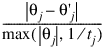
Step_Eps—Scaled step tolerance. The jth component of the scaled step from points θ and θ’ is computed as:
where t = Theta_Scale. Default: Step_Eps = ε2/ 3, where ε is machine precision
Rel_Eps_Sse—Relative SSE function tolerance. Default: Sse_Rel_Eps = max(10–10, ε2 / 3), max (10–20, ε2 / 3) in double, where ε is the machine precision
Abs_Eps_Sse—Absolute SSE function tolerance. Default: Abs_Eps_Sse = max(10 –20, ε2), max(10 –40, ε2) in double, where ε is the machine precision
Max_Step—Maximum allowable step size. Default: Max_Step = 1000 max(ε1, ε2), where ε1 = (tTθ0)1/2, ε2 = ||t||2, t = Theta_Scale, and θ0 = Theta_Guess
Trust_Region—Size of initial trust region radius. The default is based on the initial scaled Cauchy step.
N_Digit—Number of good digits in the function. Default: machine dependent
Itmax—Maximum number of iterations. Default: Itmax = 100
Max_Sse_Evals—Maximum number of SSE function evaluations. Default: Max Sse Evals = 400
Max_Jac_Evals—Maximum number of Jacobian evaluations. Default: Max Jac Evals = 400
Tolerance—False convergence tolerance. Default: Tolerance = 100 * ε, where ε is machine precision.
Output Keywords
Predicted—Named variable into which the one-dimensional array, containing the predicted values at the approximate solution, is stored.
Residual—Named variable into which the one-dimensional array, containing the residuals at the approximate solution, is stored.
R_Matrix—Named variable into which the two-dimensional array of size n_parameters × n_parameters, containing the R matrix from a QR decomposition of the Jacobian, is stored.
R_Rank—Named variable into which the rank of the R matrix is stored. A rank of less than n_parameters may indicate the model is overparameterized.
Df—Named variable into which the degrees of freedom is stored.
Sse—Named variable into which the residual sum of squares is stored.
Discussion
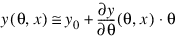
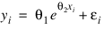
Function NONLINREGRESS fits a nonlinear regression model using least squares. The nonlinear regression model is:
yi = f(xi;θ) + εi i = 1, 2, ..., n
where the observed values of the yi’s constitute the responses or values of the dependent variable, the known xi’s are the vectors of the values of the independent (explanatory) variables, θ is the vector of p regression parameters, and the εi’s are independently distributed normal errors with mean zero and variance σ2. For this model, a least-squares estimate of θ is also a maximum likelihood estimate of θ.
The residuals for the model are as follows:
ei(θ) = yi – f(xi ; θ) i = 1, 2, ..., n
A value of θ that minimizes:
is a least-squares estimate of θ. Function NONLINREGRESS is designed so that the values of the function f(xi ; θ) are computed one at a time by a user-supplied function.
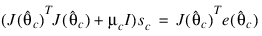
Function NONLINREGRESS is based on MINPACK routines LMDIF and LMDER by Moré et al. (1980) that use a modified Levenberg-Marquardt method to generate a sequence of approximations to a minimum point. Let:
be the current estimate of θ. A new estimate is given by:
where sc is a solution to the following:
Here:
is the Jacobian evaluated at:
The algorithm uses a “trust region” approach with a step bound of δc. A solution is first obtained for μc = 0. If:
this update is accepted; otherwise, μc is set to a positive value and another solution is obtained. The method is discussed by Levenberg (1944), Marquardt (1963), and Dennis and Schnabel (1983, pp. 129–147, 218–338).
If a user-supplied function is specified in Jacobian, the Jacobian is computed analytically; otherwise, forward finite differences are used to estimate the Jacobian numerically. In the latter case, especially if single precision is used, the estimate of the Jacobian may be so poor that the algorithm terminates at a noncritical point. In such instances, the user should either supply a Jacobian function, use the Double keyword, or do both.
Assuming a linear approximation of the model:
a covariance matrix c for the coefficients θ can be obtained from the output keywords Df=d, Sse=s, and R_Matrix=r like:
c = (s/d) * INV(TRANSPOSE(r)#r)
Programming Notes
Nonlinear regression allows substantial flexibility over linear regression because the user can specify the functional form of the model. This added flexibility can cause unexpected convergence problems for users who are unaware of the limitations of the software. Also, in many cases, there are possible remedies that may not be immediately obvious. The following is a list of possible convergence problems and some remedies. There is no one-to-one correspondence between the problems and the remedies. Remedies for some problems also may be relevant for other problems.
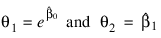
A local minimum is found. Try a different starting value. Good starting values often can be obtained by fitting simpler models. For example, for a nonlinear function:
good starting values can be obtained from the estimated linear regression coefficients:
from a simple linear regression of ln
y on
x. The starting values for the nonlinear regression in this case would be:
If an approximate linear model is not clear, then simplify the model by reducing the number of nonlinear regression parameters. For example, some nonlinear parameters for which good starting values are known could be set to these values in order to simplify the model for computing starting values for the remaining parameters.
The estimate of
θ is incorrectly returned as the same or very close to the initial estimate. This occurs often because of poor scaling of the problem, which might result in the residual sum of squares being either very large or very small relative to the precision of the computer. The keywords allow control of the scaling.
The model is discontinuous as a function of
θ. (The function
f(
x;
θ) can be a discontinuous function of
x.)
Overflow occurs during the computations. Make sure the user-supplied functions do not overflow at some value of
θ.
The estimate of
θ is going to infinity. A parameterization of the problem in terms of reciprocals may help.
Some components of
θ are outside known bounds. This can sometimes be handled by making a function that produces artificially large residuals outside of the bounds (even though this introduces a discontinuity in the model function).
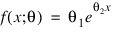
Example 1
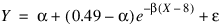
In this example (Draper and Smith 1981, p. 518), the following nonlinear model is fit:
.RUN
- FUNCTION fcn, x, theta
- RETURN, theta(0) + (0.49 - theta(0)) $
- *EXP(theta(1)*(x(0) - 8))
- END
x = [10, 20, 30, 40]
y = [0.48, 0.42, 0.40, 0.39]
n_parameters = 2
theta_hat = NONLINREGRESS('fcn', n_parameters, x, y)PRINT, 'Estimated Coefficients:', theta_hat
Example 2
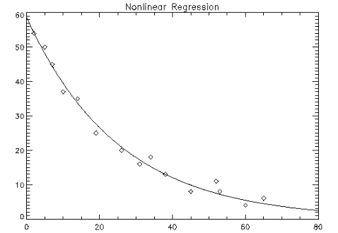
Consider the nonlinear regression model and data set discussed by Neter et al. (1983, pp. 475–478):
There are two parameters and one independent variable. The data set considered consists of 15 observations. The results are shown in
Original Data and Nonlinear Regression Fit Plot.
; Define function that defines nonlinear regression problem.
FUNCTION fcn, x, theta
RETURN, theta(0) * EXP(x(0) * theta(1))
END
; Define the Jacobian function.
FUNCTION jac, x, theta
; The following assignment produces array of correct size to
; use as the return value of the Jacobian.
fjac = theta
fjac(0) = -exp(theta(1) * x(0))
fjac(1) = -theta(0) * x(0) * EXP(theta(1) * x(0))
; Compute the Jacobian.
RETURN, fjac
END
PRO nlnreg_ex
; Define x and y.
x = [2, 5, 7, 10, 14, 19, 26, 31, 34, 38, 45, 52, 53, 60, 65]
y = [54, 50, 45, 37, 35, 25, 20, 16, 18, 13, 8, 11, 8, 4, 6]
theta_hat = NONLINREGRESS('fcn', 2, x, y, $ Theta_Guess = [60, -0.03], $
Grad_Eps = 0.001, Jacobian = 'jac')
; Plot original data.
PLOT, x, y, Psym = 4, Title = 'Nonlinear Regression'
xtmp = 80 * FINDGEN(200)/199
; Plot regression.
OPLOT, xtmp, theta_hat(0) * EXP(xtmp * theta_hat(1))
END
Informational Errors
STAT_STEP_TOLERANCE—Scaled step tolerance satisfied. The current point may be an approximate local solution, but it is also possible that the algorithm is making very slow progress and is not near a solution or that Step_Eps is too big.
Warning Errors
STAT_LITTLE_FCN_CHANGE—Both actual and predicted relative reductions in the function are less than or equal to the relative function tolerance.
STAT_TOO_MANY_ITN—Maximum number of iterations exceeded.
STAT_TOO_MANY_FCN_EVAL—Maximum number of function evaluations exceeded.
STAT_TOO_MANY_JACOBIAN_EVAL—Maximum number of Jacobian evaluations exceeded.
STAT_UNBOUNDED—Five consecutive steps have been taken with the maximum step length.
STAT_FALSE_CONVERGENCE—Iterates appear to be converging to noncritical point.
Version 2017.0
Copyright © 2017, Rogue Wave Software, Inc. All Rights Reserved.