CONLSQ Function (PV-WAVE Advantage)
Computes a least-squares constrained spline approximation.
Usage
result = CONLSQ(xdata, fdata, spacedim, constraints[, nhard])
Input Parameters
xdata—One-dimensional array containing the abscissas of the least-squares problem.
fdata—One-dimensional array containing the ordinates of the least-squares problem.
spacedim—Linear dimension of the spline subspace. It should be smaller than the number of data points and greater than or equal to the order of the spline (whose default value is 4).
constraints—Array of structures containing the abscissas at which the fit is to be constrained, the derivative of the spline that is to be constrained, the type of constraints, and any lower or upper limits.
note | To enable double precision, use double precision for all floating-point values in the constraints array of structures. |
A description of the structure fields is in the table below.

XVAL—Point at which fit is constrained (float).
DER—Derivative value of the spline to be constrained (long int).
TYPE—Types of the general constraints (long int).
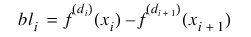
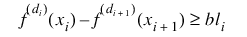
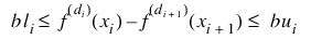
BL—Lower limit of the general constraints (float).
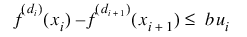
BU—Upper limit of the general constraints (float).
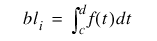
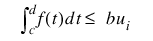
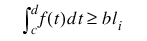
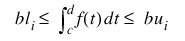
note | To constrain the integral of the spline over the closed interval (c, d), set constraints (i).XVAL = c and constraints (i + 1).XVAL = d. For consistency, insist that constraints (i).TYPE = constraints (i + 1).TYPE = 5, 6, 7, or 8 and c ≤ d. |
For more information on the allowed values of constraints.TYPE, refer to the Discussion of CONLSQ.
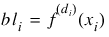
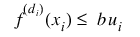
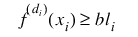
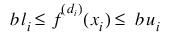
constraints(i).TYPE-th constraint
1
2
3
4
5
6
7
8
20 periodic end conditions
99 disregard this constraint
In order to have two-point constraints, constraints(i).TYPE = constraints(i + 1).TYPE is needed.
constraints(i).TYPE ith constraint
9
10
11
12
nhard—(Optional) Number of entries of constraints involved in the “hard” constraints. Note that 0 ≤ nhard ≤ (SIZE (constraints)) (1). The default, nhard = 0, always results in a fit, while setting nhard = (SIZE (constraints)) (1) forces all constraints to be met. The “hard” constraints must be met or the function signals fail. The “soft” constraints need not be satisfied, but there is an attempt to satisfy the “soft” constraints. The constraints must be listed in terms of priority with the most important constraints first. Thus, all “hard” constraints must precede “soft” constraints. If infeasibility is detected among the “soft” constraints, the function satisfies, in order, as many of the “soft” constraints as possible. Default: nhard = 0
Returned Value
result—A structure that represents the spline fit.
Input Keywords
Double—This keyword has been deprecated starting with version 10.0 of PV-WAVE. To enable double-precision, see the constraints parameter.
Order—Specifies the order of the spline. Default: Order = 4, i.e., cubic splines
Knots—Specifies the array of knots to be used when computing the spline. Default: knots are equally spaced
Weights—Array containing the weights to be used. Default: all weights equal 1
Discussion
Function CONLSQ produces a constrained, weighted, least-squares fit to data from a spline subspace. Constraints involving one-point, two-points, or integrals over an interval are allowed.
The types of constraints supported by the functions are of four types:
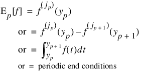
An interval, Ip, (which may be a point, a finite interval, or a semi-infinite interval) is associated with each of these constraints.
The input for this function consists of the data set (xi, fi) for i = 1, ..., N (where N = N_ELEMENTS(xdata)); that is, the data which is to be fit and the dimension of the spline space from which a fit is to be computed, spacedim. The constraints argument is an array of structures that contains the abscissas of the points involved in specifying the constraints, as well as information relating the type of constraints and the constraint interval. The optional argument nhard allows users of this code to specify which constraints must be met and which constraints can be removed in order to compute a fit. The algorithm tries to satisfy all the constraints, but if the constraints are inconsistent, then it drops constraints in the reverse order specified, until either a consistent set of constraints is found or the “hard” constraints are determined to be inconsistent (the “hard” constraints are those involving constraints(0), ..., constraints(nhard – 1)).
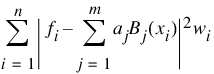
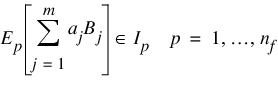
Let nf denote the number of feasible constraints as described above. The function solved the problem:
subject to:
This linearly constrained least-squares problem is treated as a quadratic program and is solved by invoking function QUADPROG.
The choice of weights depends on the data uncertainty in the problem. In some cases, there is a natural choice for the weights based on the estimates of errors in the data points.
Determining feasibility of linear constraints is a numerically sensitive task. If difficulties are encountered, a quick fix is to widen the constraint intervals Ip.
Example
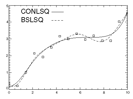
This example is a simple application of CONLSQ. Data from the function
x/2 + sin(
x/2) contaminated with random noise is generated and then fit with cubic splines. The function is increasing so it is hoped that the least-squares fit also is increasing. This is not the case for the unconstrained least-squares fit generated by function BSLSQ. The derivative is then forced to be greater than zero at 15 equally spaced points and CONLSQ is called. The resulting curve is monotone as shown in
Figure 4-13: Monotonic B-Spline Fit to Noisy Data on page 167.
; Set the random seed.
RANDOMOPT, Set = 234579
; Generate the data to be fit.
ndata = 15;
spacedim = 8;
x = 10 * FINDGEN(ndata)/(ndata - 1)
y = .5 * (x) + SIN(.5 * (x)) + RANDOM(ndata) - .5
; Compute the unconstrained least-squares fit.
sp1 = BSLSQ(x, y, spacedim)
; Define the constraints to be used by CONLSQ.
nconstraints = 15
; Define an array of constraint structures. Each element of the
; array contains one structure that defines a constraint.
constraints = REPLICATE({constraint, $ XVAL:0.0, DER:0L, TYPE:0L, BL:0.0, BU:0.0}, nconstraints)
; Put a constant at 15 equally spaced points.
constraints.XVAL = 10*FINDGEN(nconstraints)/(nconstraints - 1)
; Define constraints to force the second derivative to be greater
; than zero at the 15 equally spaced points.
FOR i=0L, nconstraints - 1 DO BEGIN &$
constraints(i).DER = 1 &$
constraints(i).TYPE = 3 &$
constraints(i).BL = 0. &$
ENDFOR
; Call CONLSQ.
sp2 = CONLSQ(x, y, spacedim, constraints)
nplot = 100
xplot = 10 * FINDGEN(nplot)/(nplot - 1)
yplot1 = SPVALUE(xplot, sp1)
yplot2 = SPVALUE(xplot, sp2)
; Plot the results.
PLOT, xplot, yplot1, Linestyle = 2
OPLOT, xplot, yplot2
OPLOT, x, y, Psym = 6
XYOUTS, 1, 4.5, 'CONLSQ', Charsize = 2
XYOUTS, 1, 4, 'BSLSQ', Charsize = 2
OPLOT, [3.6, 4.6], [4.6, 4.6]
OPLOT, [3.6, 4.6], [4.1, 4.1], Linestyle = 2
Version 2017.0
Copyright © 2017, Rogue Wave Software, Inc. All Rights Reserved.