IMSL Statistics Reference Guide > Analysis of Variance and Designed Experiments > ANOVAFACT Function (PV-WAVE Advantage)
  

ANOVAFACT Function (PV-WAVE Advantage)
Analyzes a balanced factorial design with fixed effects.
Usage
result = ANOVAFACT(n_levels, y)
Input Parameters
n_levels—One-dimensional array containing the number of levels for each of the factors and the number of replicates for each effect.
y—One-dimensional array of length:
n_levels (0) * n_levels (1) * ... * ((N_ELEMENTS (n_levels) – 1))
containing the responses. Parameter y must not contain NaN for any of its elements, i.e., missing values are not allowed.
Returned Value
result—The p-value for the overall F-test.
Input Keywords
Double—If present and nonzero, then double precision is used.
Order—Number of factors included in the highest-way interaction in the model. Order must be in the interval [1, N_ELEMENTS (n_levels) – 1]. For example, an Order of 1 indicates that a main-effect model is analyzed, and an Order of 2 indicates that two-way interactions are included in the model. Default: Order = N_ELEMENTS(n_levels) – 1)
Pure_Error, Pool_InterIf present and nonzero, Pure_Error (the default option) indicates all the main effect and the interaction effects involving the replicates, the last element in n_levels, are pooled together to create the error term. The Pool_Inter option indicates (Order + 1)-way and higher-way interactions are pooled together to create the error. Keywords Pure_Error and Pool_Inter cannot be used together.
Output Keywords
Anova_Table—Named variable into which an array of size 15 containing the analysis of variance table is stored. The analysis of variance statistics are given as follows:
*0—degrees of freedom for the model
*1—degrees of freedom for error
*2—total (corrected) degrees of freedom
*3—sum of squares for the model
*4—sum of squares for error
*5—total (corrected) sum of squares
*6—model mean square
*7—error mean square
*8—overall F-statistic
*9—p-value
*10—R2 (in percent)
*11—adjusted R2 (in percent)
*12—estimate of the standard deviation
*13—overall mean of y
*14—coefficient of variation (in percent)
Test_Effects—Named variable into which an array of size nef × 4 containing statistics relating to the sums of squares for the effects in the model is stored. Here:
where n is given by N_ELEMENTS(n_levels) if Pool_Inter is specified; otherwise, N_ELEMENTS(n_levels) – 1.
Suppose the factors are A, B, C, and error. With Order = 3, rows 0 through nef – 1 correspond to A, B, C, AB, AC, BC, and ABC. The columns of Test_Effects are as follows:
*0degrees of freedom
*1sum of squares
*2F-statistic
*3p-value
Means—Named variable into which an array of length (n_levels(0) + 1) × (n_levels(1) + 1) × ... × (n_levels(n–1) + 1) containing the subgroup means is stored.
See keyword Test_Effects for a definition of n. If the factors are A, B, C, and replicates, the ordering of the means is grand mean, A means, B means, C means, AB means, AC means, BC means, and ABC means.
Discussion
Function ANOVAFACT performs an analysis for an n-way classification design with balanced data. For balanced data, there must be an equal number of responses in each cell of the n-way layout. The effects are assumed to be fixed effects. The model is an extension of the two-way model to include n factors. The interactions (two-way, three-way, up to n-way) can be included in the model, or some of the higher-way interactions can be pooled into error. The keyword Order specifies the number of factors to be included in the highest-way interaction. For example, if three-way and higher-way interactions are to be pooled into error, set Order = 2.
By default, Order = N_ELEMENTS (n_levels) – 1 with the last subscript being the replicates subscript. Keyword Pure_Error indicates there are repeated responses within the n-way cell; Pool_Inter indicates otherwise.
Function ANOVAFACT requires the responses as input into a single vector y in lexicographical order, so that the response subscript associated with the first factor varies least rapidly, followed by the subscript associated with the second factor, and so forth. Hemmerle (1967, Chapter 5) discusses the computational method.
Example 1
A two-way analysis of variance is performed with balanced data discussed by Snedecor and Cochran (1967, Table 12.5.1, p. 347). The responses are the weight gains (in grams) of rats that were fed diets varying in the source (A) and level (B) of protein.
The model is:
for ; ;
where:
for
for i = 0, 1. The first responses in each cell in the two-way layout are given in Cell First Responses:
 
Table 5-24: Cell First Responses
Protein Level (B)
Protein Source (A)
Beef
Cereal
Pork
High
73, 102, 118, 104, 81, 107, 100, 87, 117, 111
98, 74, 56, 111, 95, 88, 82, 77, 86, 92
94, 79, 96, 98, 102, 102, 108, 91, 120, 105
Low
90, 76, 90, 64, 86, 51, 72, 90, 95, 78
107, 95, 97, 80, 98, 74, 74, 67, 89, 58
49, 82, 73, 86, 81, 97, 106, 70, 61, 82
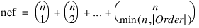
n = [3, 2, 10] 
y = [73.0, 102.0, 118.0, 104.0,  81.0, 107.0, 100.0,  87.0, $
   117.0, 111.0, 90.0,  76.0,  90.0,  64.0,  86.0, 51.0,  72.0, $
   90.0,  95.0,  78.0, 98.0,  74.0,  56.0, 111.0,  95.0, 88.0, $
   82.0, 77.0,  86.0,  92.0, 107.0,  95.0,  97.0,  80.0,  98.0, $
   74.0,  74.0,  67.0,  89.0,  58.0, 94.0,  79.0,  96.0,  98.0, $
   102.0, 102.0, 108.0, 91.0, 120.0, 105.0, 49.0,  82.0,  73.0, $
   86.0,  81.0, 97.0, 106.0, 70.0,  61.0,  82.0] 
p_value = ANOVAFACT(n, y, Anova_Table = anova_table) 
PRINT, 'p-value = ', p_value 
; PV-WAVE prints: p-value =    0.00229943
Example 2: Two-way ANOVA
In this example, the same model and data are fit as in the initial example, but keywords are used for a more complete analysis. First, a procedure to output the results is defined.
PRO print_results, anova_table, test_effects, means 
   anova_labels = ['df for among groups', $
      'df for within groups', 'total (corrected) df', $
      'ss for among groups', 'ss for within groups', $
      'total (corrected) ss', 'mean square among groups', $
      'mean square within groups', 'F-statistic', $
      'P-value', 'R-squared (in percent)', $
      'adjusted R-squared (in percent)', $
      'est. std of within group error', 'overall mean of y', $
      'coef. of variation (in percent)'] 
   effects_labels = ['A  ', 'B  ', 'A*B'] 
   means_labels = ['grand', 'A1', 'A2', $
      'A3', 'B1', 'B2', 'A1*B1', 'A1*B2', $
      'A2*B1', 'A2*B2', 'A3*B1', 'A3*B2'] 
   PRINT, '       * *Analysis of Variance * *' 
   FOR i=0L, 14 DO PM, anova_labels(i), $
      anova_table(i), Format = '(a40,f15.2)' 
   PRINT 
   ; Print the analysis of variance table. 
   PRINT, '     * * Variation Due to the Model * *' 
   PRINT, 'Source    DF      SS      MS      P-value' 
   FOR i=0L, 2 DO PM, effects_labels(i), test_effects(i, *) 
   PRINT 
   PRINT, ' * * Subgroup Means * *' 
   FOR i=0L, 11 DO PM, means_labels(i), $
      means(i), Format = '(a5,f15.2)' 
END
n = [3, 2, 10] 
y = [73.0, 102.0, 118.0, 104.0,  81.0, 107.0, 100.0,  87.0, $
   117.0, 111.0, 90.0,  76.0,  90.0,  64.0,  86.0, 51.0,  72.0, $
   90.0,  95.0,  78.0, 98.0,  74.0,  56.0, 111.0,  95.0, 88.0, $
   82.0,  77.0,  86.0,  92.0, 107.0,  95.0,  97.0,  80.0, 98.0, $
   74.0,  74.0,  67.0,  89.0,  58.0, 94.0,  79.0,  96.0,  98.0, $
   102.0, 102.0, 108.0,  91.0, 120.0, 105.0, 49.0,  82.0, 73.0, $
   86.0,  81.0, 97.0, 106.0,  70.0,  61.0,  82.0] 
p_value = ANOVAFACT(n, y, Anova_Table = anova_table, $
   Test_Effects = test_effects, Means = means) 
print_results, anova_table, test_effects, means 
This results in the following output:
* *Analysis of Variance * *
df for among groups                     5.00
df for within groups                   54.00
total (corrected) df                   59.00
ss for among groups                  4612.93
ss for within groups                11586.00
total (corrected) ss                16198.93
mean square among groups              922.59
mean square within groups             214.56
F-statistic                             4.30
P-value                                 0.00
R-squared (in percent)                 28.48
adjusted R-squared (in percent)        21.85
est. std of within group error         14.65
overall mean of y                      87.87
coef. of variation (in percent)        16.67
 * * Variation Due to the Model * * 
Source DF SS MS P-value
A  2.00000 266.533   0.621128 0.541132
B 1.00000 3168.27 14.7667    0.000322342
A*B 2.00000 1178.13   2.74552 0.0731880
 * * Subgroup Means * * 
grand          87.87 
 A1            89.60 
 A2            84.90 
 A3            89.10 
 B1            95.13 
 B2            80.60 
A1*B1         100.00 
A1*B2          79.20 
A2*B1          85.90 
A2*B2          83.90 
A3*B1          99.50 
A3*B2          78.70
Example 3: Three-way ANOVA
This example performs a three-way analysis of variance using data discussed by John (1971, pp. 91–92). The responses are weights (in grams) of roots of carrots grown with varying amounts of applied nitrogen (A), potassium (B), and phosphorus (C). Each cell of the three-way layout has one response. Note that the ABC interactions sum of squares (186) is given incorrectly by John (1971, Table 5.2.)
The three-way layout is given in Three-way Layout:
 
Table 5-25: Three-way Layout
 
A0
A1
A2
 
B0
B1
B2
B0
B1
B2
B0
B1
B2
C0
88.76
91.41
97.85
94.83
100.49
99.75
99.90
100.23
104.51
C1
87.45
98.27
95.85
84.57
97.20
112.30
92.98
107.77
110.94
C2
86.01
104.20
90.09
81.06
120.80
108.77
94.72
118.39
102.87
PRO print_results, anova_table, test_effects, means 
   anova_labels = ['df for among groups', $
      'df for within groups', 'total (corrected) df', $
      'ss for among groups', 'ss for within groups', $
      'total (corrected) ss', 'mean square among groups', $
      'mean square within groups', 'F-statistic', $
      'P-value', 'R-squared (in percent)', $
      'adjusted R-squared (in percent)', $
      'est. std of within group error', $
      'overall mean of y', 'coef. of variation (in percent)'] 
   effects_labels = ['A  ', 'B  ', 'C  ', 'A*B', 'A*B', 'A*C'] 
   PRINT, '       * *Analysis of Variance * *' 
   FOR i=0L, 14 DO PM, anova_labels(i), $
      anova_table(i), Format = '(a40,f15.2)' 
   PRINT 
   PRINT, '     * * Variation Due to the Model * *' 
   PRINT, 'Source      DF     SS       MS     P-value' 
   FOR i=0L,5 DO PM, effects_labels(i), test_effects(i, *) 
END
n = [3, 3, 3] 
y = [88.76, 87.45, 86.01, 91.41, 98.27, 104.20, 97.85, $
   95.85, 90.09, 94.83, 84.57, 81.06, 100.49, 97.20, $
   120.80, 99.75, 112.30, 108.77, 99.90, 92.98, 94.72, $
   100.23, 107.77, 118.39, 104.51, 110.94, 102.87] 
p_value = ANOVAFACT(n, y, Anova_Table = anova_table, $
   Test_Effects = test_effects, /Pool_Inter) 
print_results, anova_table, test_effects
This results in the following output:
* *Analysis of Variance * * 
df for among groups                    18.00
df for within groups                    8.00
total (corrected) df                   26.00
ss for among groups                  2395.73
ss for within groups                  185.78
total (corrected) ss                 2581.51
mean square among groups              133.10
mean square within groups              23.22
F-statistic                             5.73
p-value                                 0.01
R-squared (in percent)                 92.80
adjusted R-squared (in percent)        76.61
est. std of within group error          4.82
overall mean of y                      98.96
coef. of variation (in percent)         4.87
 * * Variation Due to the Model * * 
Source   DF      SS         MS       p-value 
A    2.00000   488.368    10.5152    0.00576699
B    2.00000  1090.66     23.4832    0.000448704
C    2.00000    49.1484    1.05823   0.391063
A*B  4.00000   142.586     1.53502   0.280423
A*B  4.00000    32.3474    0.348241  0.838336
A*C  4.00000   592.624     6.37997   0.0131252

Version 2017.0
Copyright © 2017, Rogue Wave Software, Inc. All Rights Reserved.