ANOVABALANCED Function (PV-WAVE Advantage)
Analyzes a balanced complete experimental design for a fixed, random, or mixed model.
Usage
result = ANOVABALANCED(n_levels, y, n_random, idx_rand_fct, n_fct_per_eff, idx_fct_per_eff)
Input Parameters
n_levels—One-dimensional array containing the number of levels for each of the factors.
y—One-dimensional array containing the responses. y must not contain NaN (not a number) for any of its elements, i.e., missing values are not allowed.
n_random—For positive n_random, |n_random| is the number of random factors. For negative n_random, |n_random| is the number of random effects (sources of variation).
idx_rand_fct—One-dimensional index array of length |n_random| containing either the factor numbers to be considered random (for n_random positive) or containing the effect numbers to be considered random (for n_random negative).
n_fct_per_eff—One-dimensional array containing the number of factors associated with each effect in the model.
idx_fct_per_eff—One-dimensional index array of length N_ELEMENTS(n_fct_per_effect). The first n_fct_per_eff(0) elements give the factor numbers in the first effect. The next n_fct_per_eff(1) elements give the factor numbers in the second effect. The last n_fct_per_eff(N_ELEMENTS(n_fct_per_eff)) elements give the factor numbers in the last effect. Main effects must appear before their interactions. In general, an effect E cannot appear after an effect F if all of the indices for E appear also in F.
Returned Value
result—The p-value for the F-statistic.
Input Keywords
Double—If present and nonzero, then double precision is used.
Confidence—Confidence level for two-sided interval estimates on variance components, in percent. Confidence percent confidence intervals are computed, hence, Confidence must be in the interval [0.0, 100.0]. Confidence is often 90.0, 95.0, or 99.0. For one-sided intervals with confidence level α, α in the interval [50.0, 100.0], set Confidence = 100.0 – 2.0 * (100.0 – α). Default: Confidence = 95.0
Model—Model Option

0
—Searle model (Default)
1
—Scheffe model
For Scheffe model, effects corresponding to interactions of fixed and random factors have their sum over the subscripts corresponding to fixed factors equal to zero. Also, the variance of a random interaction effect involving some fixed factors has a multiplier for the associated variance component that involves the number of levels in the fixed factors. The Searle model has no summation restrictions on the random interaction effects and has a multiplier of one for each variance component.
Output Keywords
Anova_Table—Named variable into which an array of size 15 containing the analysis of variance table is stored. The analysis of variance statistics are as follows:
0
—Degrees of freedom for the model
1
—Degrees of freedom for error
2
—Total (corrected) degrees of freedom
3
—Sum of squares for the model
4
—Sum of squares for error
5
—Total (corrected) sum of squares
6
—Model mean square
7
—Error mean square
8
—Overall
F-statistic
9
—p-value
10—
R2 (in percent)
11—adjusted
R2 (in percent)
12—estimate of the standard deviation
13—overall mean of
y14—coefficient of variation (in percent)
Var_Comp—Named variable into which an array of length N_ELEMENTS(n_fct_per_eff) + 1, by 9 array containing statistics relating to the particular variance components or effects in the model and the error is stored. Rows of Var_Comp correspond to the rows of N_ELEMENTS(n_fct_per_eff) effects plus error.
1—Degrees of freedom
2—Sum of squares
3—Mean squares
4—
F -statistic
5—
p-value for
F test
6—Variance component estimate
7—Percent of variance of
y explained by random effect
8—Lower endpoint for confidence interval on the variance component
9—Upper endpoint for confidence interval on the variance component
Columns 6 through 9 contain NaN (not a number) if the effect is fixed, i.e., if there is no variance component to be estimated. If the variance component estimate is negative, columns 8 and 9 contain NaN.
Ems—Named variable into which a one-dimensional array of length ((N_ELEMENTS(n_fct_per_eff) + 1)*(N_ELEMENTS(n_fct_per_eff) + 2))/2 containing expected mean square coefficients is stored. Suppose the effects are A, B, and AB. The ordering of the coefficients in Ems is as follows:
Y_Means—Named variable into which a one-dimensional array of length (n_levels(0) + 1) * (n_levels (1) + 1) * ... * (n_levels (n_factors – 1) + 1) containing the subgroup means is stored. Suppose the factors are A, B, and C. The ordering of the means is grand mean, A means, B means, C means, AB means, AC means, BC means, and ABC means.
Discussion
Function ANOVABALANCED analyzes a balanced complete experimental design for a fixed, random, or mixed model. The analysis includes an analysis of variance table, and computation of subgroup means and variance component estimates. A choice of two parameterizations of the variance components for the model can be made.
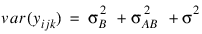
Scheffé (1959, pages 274−289) discusses the parameterization for Model = 1. For example, consider the following model equation with fixed factor A and random factor B:
yijk = μ + αi + bj + cij + eijk i = 1, 2, ..., a; j = 1, 2, ... , b; k = 1, 2, ..., n
The fixed effects αi’s are subject to the restriction:
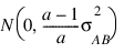
the bj’s are random effects identically and independently distributed:
cij are interaction effects each distributed:
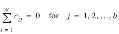
and are subject to the restrictions:
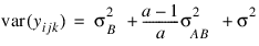
and the eijk’s are errors identically and independently distributed N(0, σ2). In general, interactions of fixed and random factors have sums over subscripts corresponding to fixed factors equal to zero. Also in general, the variance of a random interaction effect is the associated variance component times a product of ratios for each fixed factor in the random interaction term. Each ratio depends on the number of levels in the fixed factor. In the earlier example, the random interaction AB has the ratio (a – 1)/a as a multiplier of:
and:
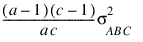
In a three-way crossed classification model, an ABC interaction effect with A fixed, B random, and C fixed would have variance:
Searle (1971, pages 400−401) discusses the parameterization for Model = 0. This parameterization does not have the summation restrictions on the effects corresponding to interactions of fixed and random factors. Also, the variance of each random interaction term is the associated variance component, i.e., without the multiplier. This parameterization is also used with unbalanced data, which is one reason for its popularity with balanced data also. In the earlier example:
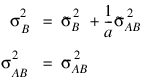
Searle (1971, pages 400−404) compares these two parameterizations. Hocking (1973) considers these different parameterizations and concludes they are equivalent because they yield the same variance-covariance structure for the responses. Differences in covariances for individual terms, differences in expected mean square coefficients and differences in F tests are just a consequence of the definition of the individual terms in the model and are not caused by any fundamental differences in the models. For the earlier two-way model, Hocking states that the relations between the two parameterizations of the variance components are:
where:
are the variance components in the parameterization with Model = 0.
Computations for degrees of freedom and sums of squares are the same regardless of the Model option. ANOVABALANCED first computes degrees of freedom and sum of squares for a full factorial design. Degrees of freedom for effects in the factorial design that are missing from the specified model are pooled into the model effect containing the fewest subscripts but still containing the factorial effect. If no such model effect exists, the factorial effect is pooled into error. If more than one such effect exists, a terminal error message is issued indicating a misspecified model.
The analysis of variance method is used for estimating the variance components. This method solves a linear system in which the mean squares are set to the expected mean squares. A problem that Hocking (1985, pages 324−330) discusses is that this method can yield a negative variance component estimate. Hocking suggests a diagnostic procedure for locating the cause of the negative estimate. It may be necessary to re-examine the assumptions of the model.
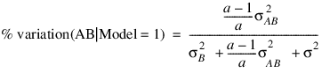
The percentage of variation explained by each random effect is computed (output in Var_Comp element 7) as variance of the associated random effect divided by variance of y. The two parameterizations can lead to different values because of the different definitions of the individual terms in the model. For example, the percentage associated with the AB interaction term in the earlier two-way mixed model is computed for Model = 1 using:
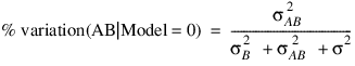
while for the parameterization Model = 0, the percentage is computed using the formula:
In each case, the variance components are replaced by their estimates (stored in Var_Comp element 6).
Confidence intervals on the variance components are computed using the method discussed by Graybill (1976, Theorem 15.3.5, page 624, and Note 4, page 620).
Example
An analysis of a generalized randomized block design is performed using data discussed by Kirk (1982, Table 6.10-1, pages 293−297). The model is:
yijk = μ + α i + bj + cij + eijk i = 1, 2, 3, 4; j = 1, 2, 3, 4; k = 1, 2
where yijk is the response for kth experimental unit in block j with treatment i; the αi’s are the treatment effects and are subject to the restriction:
the bj’s are block effects identically and independently distributed:
cij are interaction effects each distributed:
and are subject to the restrictions:
and the
eijk’s are errors, identically and independently distributed
N(0,
σ2). The interaction effects are assumed to be distributed independently of the errors. The data is given in
Table 5-29: Randomized Block Design on page 253.
PRO print_results, p, at, ems, y_means, var_comp
anova_labels = ['degrees of freedom for model', $
'degrees of freedom for error', $
'total (corrected) degrees of freedom', $
'sum of squares for model', 'sum of squares for error', $
'total (corrected) sum of squares', 'model mean square', $
'error mean square', 'F-statistic', 'p-value',$
'R-squared (in percent)', $
'adjusted R-squared (in percent)', $
'est. standard deviation of within error', $
'overall mean of y', $
'coefficient of variation (in percent)']
ems_labels = ['Effect A and Error', $
'Effect A and Effect AB', 'Effect A and Effect B', $
'Effect A and Effect A', 'Effect B and Error', $
'Effect B and Effect AB', 'Effect B and Effect B', $
'Effect AB and Error', 'Effect AB and Effect AB', $
'Error and Error']
components_labels = ['degrees of freedom for A', $
'sum of squares for A', 'mean square of A', $
'F-statistic for A', 'p-value for A', $
'Estimate of A', 'Percent Variation Explained by A', $
'95% Confidence Interval Lower Limit for A', $
'95% Confidence Interval Upper Limit for A', $
'degrees of freedom for B', 'sum of squares for B', $
'mean square of B', 'F-statistic for B', 'p-value for B', $
'Estimate of B', 'Percent Variation Explained by B', $
'95% Confidence Interval Lower Limit for B', $
'95% Confidence Interval Upper Limit for B', $
'degrees of freedom for AB', 'sum of squares for AB', $
'mean square of AB', 'F-statistic for AB', $
'p-value for AB', 'Estimate of AB', $
'Percent Variation Explained by AB', $
'95% Confidence Interval Lower Limit for AB', $
'95% Confidence Interval Upper Limit for AB', $
'degrees of freedom for Error', $
'sum of squares for Error', 'mean square of Error', $
'F-statistic for Error', 'p-value for Error', $
'Estimate of Error', 'Percent Explained by Error', $
'95% Confidence Interval Lower Limit for Error', $
'95% Confidence Interval Upper Limit for Error']
means_labels = ['Grand mean', ' A means 1', ' A means 2', $
' A means 3', ' A means 4', ' B means 1', ' B means 2', $
' B means 3', ' B means 4', 'AB means 1 1', $
'AB means 1 2', 'AB means 1 3', 'AB means 1 4', $
'AB means 2 1', 'AB means 2 2', 'AB means 2 3', $
'AB means 2 4', 'AB means 3 1', 'AB means 3 2', $
'AB means 3 3', 'AB means 3 4', 'AB means 4 1', $
'AB means 4 2', 'AB means 4 3', 'AB means 4 4']
PRINT, 'p value of F statistic =', p
PRINT
PRINT, ' * * * Analysis of Variance * * *'
FOR i=0L, 14 DO $
PM, anova_labels(i), at(i), Format = '(A40, F20.5)'
PRINT
PRINT, ' * * * Expected Mean Square Coefficients * * *'
FOR i=0L, 9 DO $
PM, ems_labels(i), ems(i), Format = '(A40, F20.2)'
PRINT
PRINT, ' * * Analysis of Variance / Variance Components * *'
k = 0
FOR i=0L, 3 DO BEGIN
FOR j=0L, 8 DO BEGIN
PM, components_labels(k), var_comp(i, j), $
Format = '(A45, F20.5)'
k = k + 1
ENDFOR
ENDFOR
PRINT
PRINT, 'means', Format = '(A20)'
FOR i=0L, 24 DO $
PM, means_labels(i), y_means(i), Format ='(A20, F20.2)'
END
y = [3.0, 6.0, 3.0, 1.0, 2.0, 2.0, 3.0, 2.0, 4.0, 5.0, 4.0, $
2.0, 3.0, 4.0, 3.0, 3.0, 7.0, 8.0, 7.0, 5.0, 6.0, 5.0, $
6.0, 6.0, 7.0, 8.0, 9.0, 10.0, 10.0, 9.0, 8.0, 11.0]
n_levels = [4, 4, 2]
indrf = [2, 3]
nfef = [1, 1, 2]
indef = [1, 2, 1, 2]
p = ANOVABALANCED(n_levels, y, 2, indrf, nfef, indef, $
Anova_Table = at, Ems = ems, Y_Means = y_means, $
Var_Comp = var_comp)
; Print the results. The output is shown at the end of this
; example.
print_results, p, at, ems, y_means, var_comp
; Add Outliners
x(0, 1) = 100.0
x(3, 4) = 100.0
x(99, 2) = -100.0
p_cov = POOLED_COV(x, n_groups, Idx_Vars = idxv, $
Idx_Cols = idxc)
PM, p_cov, Title = 'Pooled Cavariance with Outliners'
; PV-WAVE prints the following:
; Pooled Cavariance with Outliners
; 60.4264 0.304244 0.127488 -1.55551
; 0.304244 70.5257 0.167135 -0.171791
; 0.127488 0.167135 0.185188 0.0684639
; -1.55551 -0.171791 0.0684639 66.3798
r_cov = ROBUST_COV(x, n_groups, Idx_Vars = idxv, $
Idx_Cols = idxc, Percentage = percentage)
PM, r_cov, Title = 'Robust Covariance with Outliners'
; PV-WAVE prints the following:
; Robust Covariance with Outliners
; 0.255521 0.0876029 0.155279 0.0359198
; 0.0876029 0.112674 0.0545391 0.0322426
; 0.155279 0.0545391 0.172263 0.0412149
; 0.0359198 0.0322426 0.0412149 0.0424182
Output
The following output is the result of this print command:
print_results, p, at, ems, y_means, var_comp
% ANOVABALANCED: Note: STAT_ENDPNTS_NEGATIVE
One or more endpoints are negative and are set to zero.
p value of F statistic = 4.94719e-06
* * * Analysis of Variance * * *
degrees of freedom for model 15.00000
degrees of freedom for error 16.00000
total (corrected) degrees of freedom 31.00000
sum of squares for model 216.50000
sum of squares for error 19.00000
total (corrected) sum of squares 235.50000
model mean square 14.43333
error mean square 1.18750
F-statistic 12.15439
p-value 0.00000
R-squared (in percent) 91.93206
adjusted R-squared (in percent) 84.36836
est. standard deviation of within error 1.08972
overall mean of y 5.37500
coefficient of variation (in percent) 20.27395
* * * Expected Mean Square Coefficients * * *
Effect A and Error 1.00
Effect A and Effect AB 2.00
Effect A and Effect B 0.00
Effect A and Effect A 8.00
Effect B and Error 1.00
Effect B and Effect AB 2.00
Effect B and Effect B 8.00
Effect AB and Error 1.00
Effect AB and Effect AB 2.00
Error and Error 1.00
* * Analysis of Variance / Variance Components * *
degrees of freedom for A 3.00000
sum of squares for A 194.50000
mean square of A 64.83334
F-statistic for A 32.87324
p-value for A 0.00004
Estimate of A NaN
Percent Variation Explained by A NaN
95% Confidence Interval Lower Limit for A NaN
95% Confidence Interval Upper Limit for A NaN
degrees of freedom for B 3.00000
sum of squares for B 4.25000
mean square of B 1.41667
F-statistic for B 0.71831
p-value for B 0.56566
Estimate of B -0.06944
Percent Variation Explained by B 0.00000
95% Confidence Interval Lower Limit for B NaN
95% Confidence Interval Upper Limit for B NaN
degrees of freedom for AB 9.00000
sum of squares for AB 17.75000
mean square of AB 1.97222
F-statistic for AB 1.66082
p-value for AB 0.18016
Estimate of AB 0.39236
Percent Variation Explained by AB 24.83516
95% Confidence Interval Lower Limit for AB 0.00000
95% Confidence Interval Upper Limit for AB 2.75803
degrees of freedom for Error 16.00000
sum of squares for Error 19.00000
mean square of Error 1.18750
F-statistic for Error NaN
p-value for Error NaN
Estimate of Error 1.18750
Percent Explained by Error 75.16483
95% Confidence Interval Lower Limit for Error 0.65868
95% Confidence Interval Upper Limit for Error 2.75057
means
Grand mean 5.38
A means 1 2.75
A means 2 3.50
A means 3 6.25
A means 4 9.00
B means 1 6.00
B means 2 5.12
B means 3 5.12
B means 4 5.25
AB means 1 1 4.50
AB means 1 2 2.00
AB means 1 3 2.00
AB means 1 4 2.50
AB means 2 1 4.50
AB means 2 2 3.00
AB means 2 3 3.50
AB means 2 4 3.00
AB means 3 1 7.50
AB means 3 2 6.00
AB means 3 3 5.50
AB means 3 4 6.00
AB means 4 1 7.50
AB means 4 2 9.50
AB means 4 3 9.50
AB means 4 4 9.50
Version 2017.0
Copyright © 2017, Rogue Wave Software, Inc. All Rights Reserved.