SPLIT_SPLIT_PLOT Function (PV-WAVE Advantage)
Analyzes data from split-split-plot experiments. The whole-plots can be assigned to experimental units using either a completely randomized or randomized complete block design. SPLIT_SPLIT_PLOT also analyzes split-split-plot experiments replicated at several locations.
Usage
result = SPLIT_SPLIT_PLOT(n, n_locations, n_whole, n_split, n_sub, rep, whole, split, sub, y)
Input Parameters
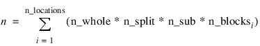
n—Number of missing and non-missing experimental observations. SPLIT_SPLIT_PLOT verifies that:
where N_blocksi is equal to the number of blocks or replicates at the ith location.
n_locations—Number of locations. n_locations must be one or greater. If n_locations > 1 then the Locations keyword must be included as input. See the Locations keyword.
n_whole—Number of levels associated with the whole-plot factor. n_whole must be greater than one.
n_split—Number of levels associated with the split-plot factor. n_split must be greater than one.
n_sub—Number of levels associated with the sub-plot factor. n_sub must be greater than one.
rep—Array of length n containing the block, or replicate, identifiers for each observation in y. Different locations can have different numbers of blocks or replicates. Each block or replicate at a single location must be assigned a different identifier, but different locations can have the same assignments.
whole—Array of length n containing the whole-plot identifiers for each observation in y. Each level of the whole-plot factor must be assigned a different integer. SPLIT_SPLIT_PLOT verifies that the number of unique whole-plot identifiers is equal to n_whole.
split—Array of length n containing the split-plot identifiers for each observation in y. Each level of the split-plot factor must be assigned a different integer. SPLIT_SPLIT_PLOT verifies that the number of unique split-plot identifiers is equal to n_split.
sub—Array of length n containing the sub-plot identifiers for each observation in y. Each level of the sub-plot factor must be assigned a different integer. SPLIT_SPLIT_PLOT verifies that the number of unique sub-plot identifiers is equal to n_sub.
y—Array of length n containing the experimental observations and any missing values. Missing values cannot be omitted. They are indicated by placing a NaN (Not a Number) at the appropriate positions in y. NaN can be defined by calling the MACHINE function. For example:
x = MACHINE(/Float)
y(i) = x.NaN
The location, whole-plot, split-plot and sub-plot for each observation in y are identified by the corresponding values in the input parameters whole, split, and sub and the Locations keyword.
Returned Value
result—A two dimensional, 20 by 6 array containing the ANOVA table. Each row in this array contains values for one of the effects in the ANOVA table. The first value in each row,
anova_tablei,0 =
anova_table(
i,0), identifies the source for the effect associated with values in that row. The remaining values in a row contain the ANOVA table values using the convention found in
ANOVA Table Values.
The Source Identifiers in the first column of
anova_tablei,j are the only negative values in
anova_table. Assignments of identifiers to ANOVA sources use the coding shown in
ANOVA Source Identifiers.
Input Keywords
Double—If present and nonzero, double precision is used.
Locations—Array of length n containing the location identifiers for each observation in y. Unique integers must be assigned to each location in the study. This keyword is required when n_locations > 1.
Crd—If set and nonzero, then the whole-plot factor is randomized to whole-plot experimental units. By default, the whole-plot factor is a fixed effect.
Output Keywords
N_missing—Number of missing values, if any, found in y. Missing values are denoted with a NaN (Not a Number) value.
Cv—Array of length 3 containing the whole-plot, split-plot, and sub-plot coefficients of variation. Cv(0) contains the whole-plot C.V., Cv(1) contains the split-plot C.V., and Cv(2) contains the sub-plot C.V.
Grand_mean—Mean of all the data across every location.
Whole_plot_means—Array of length n_whole containing the whole-plot means.
Split_plot_means—Array of length n_split containing the split-plot means.
Sub_plot_means—Array of length n_sub containing the sub-plot means.
Whole_split_plot_means—A 2-dimensional array of size n_whole by n_split containing the whole-plot by split-plot means.
Whole_sub_plot_means—A 2-dimensional array of size n_whole by n_sub containing the whole-plot by sub-plot means.
Split_sub_plot_means—A 2-dimensional array of size n_split by n_sub containing the split-plot by sub-plot means.
Treatment_means—Array of size (n_whole by n_split by n_sub) containing the treatment means. For i > 0, j > 0, and k > 0, Treatment_means(i,j,k) contains the mean of the observations, averaged over all locations, blocks, and replicates, for the kth sub plot within the jth split-plot within the ith whole-plot.
Std_errors—Array of length 8 containing four standard errors and their associated degrees of freedom. The standard errors are in the first four elements and their associated degrees of freedom are reported in
Std_errors(4) through
Std_errors(7). Refer to
Standard Errors for a list of the standard errors and their associated degrees of freedom.
N_blocks—Array of length n_locations containing the number of blocks, or replicates, at each location.
Location_anova_table—A 3-dimensional array of size n_locations by 20 by 6 containing the ANOVA tables associated with each location. For each location, the 20 by 6 dimensional array corresponds to the ANOVA table for that location. For example, Location_anova_table(i,j,k) contains the value in the kth column and jth row of the returned ANOVA table for the ith location.
Anova_row_labels—Array containing the labels for each of the rows of the returned ANOVA table. The label for the ith row of the ANOVA table can be printed with PRINT, Anova_row_labels(i).
Discussion
SPLIT_SPLIT_PLOT is capable of analyzing a wide variety of split-split-plot experiments.
Split-split-plot experimental designs can vary in the assignment of whole-plot factors to experimental units. In some cases, this assignment is completely random. For example, in a drug study the experimental unit might be the subject receiving a treatment. The whole-plot factor, possibly different treatments, could be assigned in one of two ways. Each subject could receive only one treatment or each could receive all treatments over an appropriate period of time. If each subject received only a single randomly selected treatment, then this design constitutes a CRD for the whole-plot factor, and the Crd keyword must be set.
On the other hand, if each subject receives every treatment in random order, then the subject is a blocking factor, and this sampling scheme constitutes an RCBD. In this case, it is necessary to assume that there are no carry-over effects from one treatment to another. This sampling scheme is the default setting.
This randomization choice occurs often in agricultural field trials. A trial designed to test different fertilizers and different seed lots can be conducted in one of two ways. The whole-plot factor, fertilizer, can be applied to different fields, or each can be applied to sub-divisions of these fields. In either case, a field, or a sub-division of a field, is the whole-plot experimental unit. In the first case, in which only one randomly selected fertilizer is applied to each field, the whole-plot factor is not blocked and this scheme is called as a CRD, and the Crd keyword must be set. However, if fertilizers are applied to sub-divisions within a field, then the whole-plot factor is blocked within fields and this assignment is referred to as an RCBD. By default, SPLIT_SPLIT_PLOT assumes that levels of the whole-plot factor are randomly assigned within blocks.
The essential distinction between split-plot and split-split-plot experiments is the presence of a third factor that is blocked, or nested, within each level of the whole-plot and split-plot factors. This third factor is referred to as the sub-plot factor.
Contrast the split-split plot experiment to the same experiment run using a strip-split plot design, see
Strip-Split Plot Experiment—Split-Plots Nested Within Strip-Plot Factors A and B. In a strip-split plot experiment factor B is applied in strip across factor A; whereas, in a split-split plot experiment, factor B is randomly assigned to each level of factor A. In a strip-split plot experiment, the level of factor B is constant across a row; whereas in a split-split plot experiment, the levels of factor B change as you go across a row, reflecting the fact that factor B is randomized within each level of factor A.
In some studies, a split-split-plot experiment is replicated at several locations. SPLIT_SPLIT_PLOT can analyze these, even when the number of blocks or replicates at each location is different. If only a single replicate or block is used at each location, then location should be treated as a blocking factor, with n_locations set equal to one. If n_locations = 1, it is assumed that the experiment was conducted at a single location with more than one block or replicate at that location. In this case, all entries in the ANOVA table associated with location will contain missing values.
However, if n_locations > 1, it is assumed the experiment was repeated at multiple locations, with replication or blocking occurring at each location. Although the number of blocks, or replicates, at each location can be different, the number of levels for whole-plot and split-plot factors, n_whole and n_split, must be the same at each location. The locations associated with each of the observations in y are specified in the keyword Locations, which is a required input keyword when n_locations > 1.
By default, locations are assumed to be random effects. Tests involving whole-plots use the interaction between whole-plots and locations as the error term for testing whether there are statistically significant differences among whole-plot factor levels. This assumes that the interaction of whole-plots and locations is not statistically significant. A test of this assumption uses the pooled whole-plot error. If the interaction between location and whole-plots, split-plots or sub-plot is statistically significant, then the nature of that interaction should be explored since it impacts the interpretation of the significance of the treatment factors.
When n_locations > 1 are assumed to be random effects, tests involving split-plots do not use the split-plot errors pooled across locations. Instead, the error term for split plots is the interaction between locations and split-plots. The split-plot by whole-plot interaction is tested against the location by split-plot by whole-plot interaction.
Suppose, for example, that a researcher wanted to conduct an agricultural experiment comparing the effectiveness of 4 fertilizers with 3 rates of application and 2 seed lots. One replicate of the experiment is conducted at each of the 3 farms. That is, only a single field at each location is assigned to this experiment.
Each field is divided into 4 whole-plots and the fertilizers are randomly assigned to each of the 4 whole-plots. Each whole-plot is then further sub-divided into 3 split-plots which are each randomly assigned one of the three fertilizer application rates. Finally, each of these sub-divisions assigned a particular fertilizer and application rate is sub-divided into 2 plots and randomly assigned one of the two seed lots.
In this case, each farm is a blocking factor, fertilizers are whole-plots and fertilizer application rate are split plots, and seed lots are sub-plots. The input array rep would contain integers from 1 to the number of farms, with n_whole = 4, n_split = 3 and n_sub = 2.
However, if each farm allocated more than a single field for this study, then each farm would be treated as a different location with n_locations set equal to the number of farms, and fields might be treated as blocking factor. The array rep would contain integers from 1 to the number fields used in a farm, and the Locations keyword must contain integers from 1 to the number of farms.
In summary SPLIT_SPLIT_PLOT can analyze 3x2=6 different experimental situations, depending upon the settings of:

Locations (none, fixed or random): specified by setting
n_locations and the
Locations keyword.
Whole-plot sampling (CRD or RCBD): specified by setting the
Crd keyword. CRD if the
Crd keyword is set, RCBD if the
Crd keyword is not set or set to 0.
The default condition depends upon the value for n_locations. If n_locations > 1, locations are assumed to be a random effect. Assignment of experimental units to whole-plots is assumed to use a RCBD design and whole-plots, split-plots, and sub-plots are all assumed to be fixed effects.
Example
This example uses data from a split-split plot design consisting of 2 whole-plots, 2-split-plots and 2 sub-plots.
; Total number of observations
n = 24
; Number of locations
n_locations = 1
; Number of Whole-plots within a location
n_whole = 2
; Number of Split-plots within a location, Whole_plot
n_split = 2
n_sub = 2
rep = [1, 1, 1, 1, 1, 1, 1, 1, $
2, 2, 2, 2, 2, 2, 2, 2, $
3, 3, 3, 3, 3, 3, 3, 3]
whole = [1, 1, 1, 1, 2, 2, 2, 2, $
1, 1, 1, 1, 2, 2, 2, 2, $
1, 1, 1, 1, 2, 2, 2, 2]
split = [1, 1, 2, 2, 1, 1, 2, 2, $
1, 1, 2, 2, 1, 1, 2, 2, $
1, 1, 2, 2, 1, 1, 2, 2]
sub = [1, 2, 1, 2, 1, 2, 1, 2, $
1, 2, 1, 2, 1, 2, 1, 2, $
1, 2, 1, 2, 1, 2, 1, 2]
y = [30.0, 40.0, 38.9, 38.2, $
41.8, 52.2, 54.8, 58.2, $
20.5, 26.9, 21.4, 25.1, $
26.4, 36.7, 28.9, 35.9, $
21.0, 25.4, 24.0, 23.3, $
34.4, 41.0, 33.0, 34.9]
aov = SPLIT_SPLIT_PLOT(n, n_locations, n_whole, n_split, $
n_sub, rep, whole, split, sub, y, $
Crd=crd, N_missing=n_missing, $
Cv=cv, Grand_mean=grand_mean, $
Whole_plot_means=whole_plot_means, $
Split_plot_means=split_plot_means, $
Sub_plot_means=sub_plot_means, $
Whole_split_plot_means= $
Whole_split_plot_means, $
Whole_sub_plot_means= $
Whole_sub_plot_means, $
Split_sub_plot_means= $
Split_sub_plot_means, $
Treatment_means=treatment_means, $
Std_errors=std_errors, $
N_blocks=n_blocks, $
Location_anova_table= $
location_anova_table )
labels = ['Location ', $
'Block Within ', $
' Location ', $
'Whole-Plot ', $
'Location x ', $
' Whole-Plot ', $
'Whole-Plot Error ', $
'Split-Plot ', $
'Location x ', $
' Split-Plot ', $
'Whole-Plot x ', $
' Split-Plot ', $
'Location x ', $
' Whole-Plot x ', $
' Split-Plot ', $
'Split-Plot Error ', $
'Sub-Plot ', $
'Location x Sub-Plot ', $
'Whole-Plot x ', $
' Sub-Plot ', $
'Location x ', $
' Whole-Plot x ', $
' Sub-Plot ', $
'Split-plot x ', $
' Sub-Plot ', $
'Location x ', $
' Split-Plot x ', $
' Sub-Plot ', $
'Whole_plot x ', $
' Split-Plot x ', $
' Sub-Plot ', $
'Location x ', $
' Whole-Plot x ', $
' Split Plot x ', $
' Sub-Plot ', $
'Sub-Plot Error ', $
'Corrected Total ']
; Print Analysis of Variance Table
PRINT, " *** ANALYSIS OF VARIANCE TABLE ***"
PRINT, 'ID', 'DF', 'SSQ', 'MS', 'F-Test', 'p-Value', $
Format='(A24, A5, A9, A8, A7, A8)'
idx = 0
FOR i=0L, (SIZE(aov))(1)-1 DO BEGIN & $
PRINT, labels(idx), aov(i,0), aov(i,1), aov(i,2), $
aov(i,3), aov(i,4), aov(i,5), Format= $
'(A20, 1X, I3, 2X, F3.0, 2X, F7.2, 2X, F6.2, 2X, ' + $
'F5.2, 2X, F6.3)' & $
idx = idx + 1 & $
IF idx LT N_ELEMENTS(labels)-1 THEN $
WHILE STRPOS(labels(idx), ' ', 0) EQ 0 DO BEGIN & $
PRINT, labels(idx) & idx = idx + 1 & $
ENDWHILE & $
ENDFOR
PRINT, ''
PRINT, grand_mean, Format="('Grand mean: ', F9.6, '\012')"
PRINT, "Coefficient of Variation"
labels = ['Whole-Plot:', 'Split-Plot:','Sub-Plot :']
FOR i=0L, 2 DO PRINT, labels(i), cv(i), Format='(A13, F9.4)'
PRINT, ''
; Print the Treatment Means
PRINT, "Treatment Means"
idx = 0
FOR i=0L, n_whole-1, idx+1 DO $
FOR j=0L, n_split-1 DO $
FOR k=0L, n_sub-1 DO $
PRINT, (i), (j), (k), treatment_means(i,j,k), $
Format="(' Treatment[', I1, ']" + $ "[', I1, '][', I1, '] Mean:', F8.4)"
PRINT, ''
PRINT, std_errors(3), $
Format='("Standard Error for Comparing Two ' + $ 'Treatment Means:", F9.6)'
PRINT, std_errors(7), Format="('(df=', F8.6, ')', '\012')"
; Perform multiple comparison using the LSD procedure
equal_means = MULTICOMP(REFORM(treatment_means, $
(n_whole*n_split*n_sub)), $
std_errors(7), std_errors(3)/SQRT(2), /LSD, $
Alpha=0.05)
PM, "LSD Comparison for Treatment Means (alpha=0.05)"
PM, equal_means, Title="Size of Groups of Means"
PM, ''
; Print the Whole-plot Means
PM, whole_plot_means, Title="Whole-plot Means"
PRINT, ''
PRINT, std_errors(0), $
Format='("Standard Error for Comparing Two ' + $ 'Whole-Plot Means:", F9.6)'
PRINT, std_errors(4), Format="('(df=', F8.6, ')', '\012')"
; Perform multiple comparison using the LSD procedure
equal_means = MULTICOMP(whole_plot_means, $
std_errors(4), std_errors(0)/SQRT(2), /LSD, $
Alpha=0.05)
PM, "LSD Comparison for Whole-Plot Means (alpha=0.05)"
PM, equal_means, Title="Size of Groups of Means"
PM, ''
; Print the Split-plot Means
PM, split_plot_means, Title="Split-plot Means"
PRINT, ''
PRINT, std_errors(1), $
Format='("Standard Error for Comparing Two ' + $ 'Split-Plot Means:", F9.6)'
PRINT, std_errors(5), Format="('(df=', F8.6, ')', '\012')"
; Perform multiple comparison using the LSD procedure
equal_means = MULTICOMP(split_plot_means, $
std_errors(5), std_errors(1)/SQRT(2), /LSD, $
Alpha=0.05)
PM, "LSD Comparison for Split-Plot Means (alpha=0.05)"
PM, equal_means, Title="Size of Groups of Means"
PRINT, ''
; Print the Sub-plot Means
PM, sub_plot_means, Title="Sub-plot Means"
PRINT, ''
PRINT, std_errors(2), $
Format='("Standard Error for Comparing Two ' + $ 'Sub-Plot Means:", F9.6)'
PRINT, std_errors(6), Format="('(df=', F8.6, ')', '\012')"
; Perform multiple comparison using the LSD procedure
equal_means = MULTICOMP(sub_plot_means, $
std_errors(6), std_errors(2)/SQRT(2), /LSD, $
Alpha=0.05)
PM, "LSD Comparison for Sub-Plot Means (alpha=0.05)"
PM, equal_means, Title="Size of Groups of Means"
Output
*** ANALYSIS OF VARIANCE TABLE ***
ID DF SSQ MS F-Test p-Value
Location -1 NaN NaN NaN NaN NaN
Block Within -2 2. 1310.28 655.14 30.82 0.031
Location
Whole-Plot -3 1. 858.01 858.01 40.37 0.024
Location x -4 NaN NaN NaN NaN NaN
Whole-Plot
Whole-Plot Error -5 2. 42.51 21.26 0.86 0.490
Split-Plot -6 1. 17.17 17.17 0.69 0.452
Location x -7 NaN NaN NaN NaN NaN
Split-Plot
Whole-Plot x -8 1. 1.55 1.55 0.06 0.815
Split-Plot
Location x -9 NaN NaN NaN NaN NaN
Whole-Plot x
Split-Plot
Split-Plot Error -10 4. 99.32 24.83 7.62 0.008
Sub-Plot -11 1. 163.80 163.80 50.27 0.000
Location x Sub-Plot -12 NaN NaN NaN NaN NaN
Whole-Plot x -13 1. 11.34 11.34 3.48 0.099
Sub-Plot
Location x -14 NaN NaN NaN NaN NaN
Whole-Plot x
Sub-Plot
Split-plot x -15 1. 46.76 46.76 14.35 0.005
Sub-Plot
Location x -16 NaN NaN NaN NaN NaN
Split-Plot x
Sub-Plot
Whole_plot x -17 1. 0.51 0.51 0.16 0.703
Split-Plot x
Sub-Plot
Location x -18 NaN NaN NaN NaN NaN
Whole-Plot x
Split Plot x
Sub-Plot
Sub-Plot Error -19 8. 26.07 3.26 NaN NaN
Corrected Total -20 23. 2577.33 NaN NaN NaN
Grand mean: 33.870834
Coefficient of Variation
Whole-Plot: 13.6116
Split-Plot: 14.7118
Sub-Plot : 5.3293
Treatment Means
Treatment[0][0][0] Mean: 23.8333
Treatment[0][0][1] Mean: 30.7667
Treatment[0][1][0] Mean: 28.1000
Treatment[0][1][1] Mean: 28.8667
Treatment[1][0][0] Mean: 34.2000
Treatment[1][0][1] Mean: 43.3000
Treatment[1][1][0] Mean: 38.9000
Treatment[1][1][1] Mean: 43.0000
Standard Error for Comparing Two Treatment Means: 1.473846
(df=8.000000)
LSD Comparison for Treatment Means (alpha=0.05)
Size of Groups of Means
0
3
0
0
0
0
2
Whole-plot Means
27.8917
39.8500
Standard Error for Comparing Two Whole-Plot Means: 2.661792
(df=2.000000)
LSD Comparison for Whole-Plot Means (alpha=0.05)
Size of Groups of Means
0
Split-plot Means
33.0250
34.7167
Standard Error for Comparing Two Split-Plot Means: 2.876944
(df=4.000000)
LSD Comparison for Split-Plot Means (alpha=0.05)
Size of Groups of Means
2
Sub-plot Means
31.2583
36.4833
Standard Error for Comparing Two Sub-Plot Means: 1.473846
(df=8.000000)
LSD Comparison for Sub-Plot Means (alpha=0.05)
Size of Groups of Means
0
Version 2017.0
Copyright © 2017, Rogue Wave Software, Inc. All Rights Reserved.