YATES Function (PV-WAVE Advantage)
Estimates missing observations in designed experiments using Yate’s method.
Usage
result = YATES(x)
Input/Output Parameters
x—A n by (n_independent + 1) 2-dimensional array containing the experimental observations and missing values. The first n_independent columns contain values for the independent variables and the last column contains the corresponding observations for the dependent variable or response. The columns assigned to the independent variables should not contain any missing values. Missing values are included in this array by placing a NaN (not a number) in the last column of x. For example:
m = MACHINE(/Float)
x(i) = m.NaN
Upon successful completion, missing values are replaced with estimates calculated using Yates’ method.
Returned Value
result—The number of missing values replaced with estimates using the Yates procedure. A negative return value indicates that the routine was unable to successfully estimate all missing values. Typically this occurs when all of the observations for a particular treatment combination are missing. In this case, Yate’s missing value method does not produce a unique set of missing value estimates.
Input Keywords
Double—If present and nonzero, double precision is used.
Design—An integer indicating whether a custom or standard design is being used. The association of values for this variable and standard designs is described in the
Design Values.
Initial_estimates—Initial estimates for the missing values. The Initial_estimates keyword is an array of length n_missing containing the initial estimates. Default: For Design = 0 and Design = 1, the initial estimates are calculated using the Yates formula for those designs. For Design = 2, the mean of the non-missing observations is used as the initial estimate for all missing values.
Itmax—Maximum number of iterations in the optimization routine for finding the missing value estimates that minimize the error sum of squares in the analysis of variance. Default: Itmax = 500.
Grad_tol—Scaled gradient tolerance used to determine whether the difference between the error sum of squares is small enough to stop the search for missing value estimates. Default: Grad_tol = ε2/3, where ε is the machine precision.
Step_tol—Scaled step tolerance used to determine whether the difference between missing value estimates is small enough to stop the search for missing value estimates. Default: step_tol = ε2/3, where ε is the machine precision.
Get_ss—Scalar string specifying the name of the PV-WAVE user-supplied function to compute the error sum of squares calculated using the n by (n_independent + 1) matrix dataMatrix. Get_ss is required input when Design = 2. The Get_ss function accepts the following parameters:
 n
n—Number of rows in
dataMatrix.
n_independent—Length of
n_levels.
n_levels—An array of length
n_independent containing the number of levels associated with each of the first
n_independent columns in
dataMatrix.
dataMatrix—Copy of
x with missing values replaced by estimates.
Output Keywords
Missing_index—Array of length n_missing containing the indices for the missing values in x. The number of missing values, n_missing, is the return value of YATES.
Error_ss—The value of the error sum of squares calculated using the missing value estimates. If Design = 2 then this is equal to the value returned from Get_ss using the Yates missing value estimates.
Discussion
Several functions for analysis of variance require balanced experimental data, i.e. data containing no missing values within a block and an equal number of replicates for each treatment. If the number of missing observations in an experiment is smaller than the Yates method as described in Yates (1933) and Steel and Torrie (1960), can be used to estimate the missing values. Once the missing values are replaced with these estimates, the data can be passed to an analysis of variance that requires balanced data.
The basic principle behind the Yates method for estimating missing observations is to replace the missing values with values that minimize the error sum of squares in the analysis of variance. Since the error sum of squares depends upon the underlying model for the analysis of variance, the Yates formulas for estimating missing values vary from ANOVA to ANOVA.
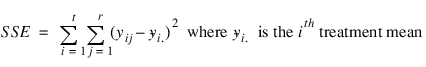
Consider, for example, the model underlying experiments conducted using a completely randomized design. If yij is the ith observation for the ith treatment then the error sum of squares for a CRD is calculated using the following formula:
If an observation yij is missing then SSE is minimized by replacing that missing observation with the estimate:
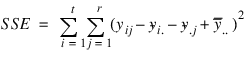
For a randomized complete block design (RCBD), the calculation for estimating a single missing observation can be derived from the RCBD error sum of squares:
If only a single observation, yij, is missing from the jth block and ith treatment, the estimate for this missing observation can be derived by solving the equation:
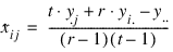
The solution is referred to as the Yates formula for a RCBD:
where:
r = number of blocks
t = number of treatments
yi = total of all non-missing observations from the
ith treatment
y.j = total of all non-missing observations from the
jth block
y = total of all non-missing observations
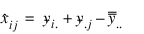
If more than one observation is missing, YATES minimization procedure is used to estimate missing values. For a CRD, all missing observations are set equal to their corresponding treatment means calculated using the non-missing observations. That is,

.
For RCBD designs with more than one missing value, Yate’s formula for estimating a single missing observation is used to obtain initial estimates for all missing values. These are passed to a function minimization routine to obtain the values that minimize SSE.
For other designs, specify Design = 2 and Get_ss. The function Get_ss is used to obtain the Yates missing value estimates by selecting the estimates that minimize sum of squares returned by Get_ss. When called, Get_ss calculates the error sum of squares at each iteration assuming that the data matrix it receives is balanced and contains no missing values.
Example
Missing values can occur in any experiment. Estimating missing values via the Yates method is usually done by minimizing the error sum of squares for that experiment. If only a single observation is missing and there is an analytical formula for calculating the error sum of squares then a formula for estimating the missing value is fairly easily derived. Consider for example a split-plot experiment with a single missing value.
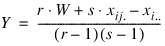
Suppose, for example, that xijk, the observation for the ith whole-plot, jth split plot and kth block is missing. Then the estimate for a single missing observation in the ith whole plot is equal to:
where:
r = number of blocks
s = number of split-plots
W = total of all non-missing values in same block as the missing observation
xij. = total of the non-missing observations across blocks of observations from
ith whole-plot factor level and the
jth split-plot level,
xi.. = the total of all observations, across split-plots and blocks of the nonmissing observations for the
ith whole plot.
If more than a single observation is missing, then an iterative solution is required to obtain missing value estimates that minimize the error sum of squares.
YATES simplifies this procedure. Consider, for example, a split-plot experiment conducted at a single location using fixed-effects whole and split plots. If there are no missing values, then the error sum of squares can be calculated from a 3-way analysis of variance using whole-plot, split-plot and blocks as the 3 factors. For balanced data without missing values, the errors sum of squares would be equal to the sum of the 3-way interaction between these factors and the split-plot by block interaction.
Calculating the error sum of squares using this 3-way analysis of variance is achieved using the ANOVAFACT routine.
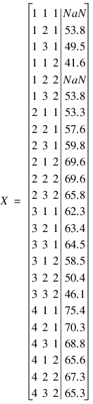
The name of the function to calculate the error sum of squares is passed to YATES using the Get_ss keyword, together with a matrix containing the data for the split-plot experiment. For this example, the following data obtained from an agricultural experiment will be used. In this experiment, 4 whole plots were randomly assigned to two 2 blocks. Whole-plots were subdivided into 2 split-plots. The whole-plot factor consisted of 4 different seed lots, and the split-plot factor consisted of 2 seed protectants. The data of this example is a 24 by 4 matrix with two missing observations.
The following program uses this data with YATES to replace the two missing values with Yates estimates.
FUNCTION get_ss,n, n_independent, n_levels, x
; Copy responses from the last column of x into a 1-D array
; as expected by ANOVAFACT.
responses = x(*, n_independent)
pvalue = ANOVAFACT(n_levels, responses, $
Test_effects=test_effects, $
Anova_table=anova_table, /Pool_Inter)
; Compute and return the error sum of squares.
errorSS = anova_table(4) + test_effects(5,1)
RETURN, errorSS
END
PRO yates_ex1
whole = [1, 1, 1, 1, 1, 1,$
2, 2, 2, 2, 2, 2,$
3, 3, 3, 3, 3, 3,$
4, 4, 4, 4, 4, 4]
split = [1, 2, 3, 1, 2, 3, $
1, 2, 3, 1, 2, 3, $
1, 2, 3, 1, 2, 3, $
1, 2, 3, 1, 2, 3]
block = [1, 1, 1, 2, 2, 2, $
1, 1, 1, 2, 2, 2, $
1, 1, 1, 2, 2, 2, $
1, 1, 1, 2, 2, 2]
y = [0.0, 53.8, 49.5, 41.6, 0.0, 53.8, $
53.3, 57.6, 59.8, 69.6, 69.6, 65.8, $
62.3, 63.4, 64.5, 58.5, 50.4, 46.1, $
75.4, 70.3, 68.8, 65.6, 67.3, 65.3]
; Set the first and fifth observations to missing values.
amach = MACHINE(/Float)
y(0) = amach.NAN
y(4) = amach.NAN
; Fill the array x with the classification variables
; and observations.
x = [[whole],[split],[block],[y]]
; Sort the data since ANOVAFACT will expect sorted data.
x = SORTDATA(x, 3)
result = YATES(x, $
Get_ss = 'get_ss', $
Design = 2, $
Missing_index = missing_index, $
Error_ss = error_ss, $
Itmax = 500)
; Output results
PRINT, "Returned error sum of squares: ", error_ss
PRINT, "Missing values replaced: ", result
PM, x(missing_index, *), Title = "Rows of x with estimates"
PM, x, Title = "Sorted x, with estimates"
END
Output
Returned error sum of squares: 95.6200
Missing values replaced: 2
Rows of x with estimates
1.00000 1.00000 1.00000 37.2992
1.00000 2.00000 2.00000 58.1007
Sorted x, with estimates
1.00000 1.00000 1.00000 37.2992
1.00000 1.00000 2.00000 41.6000
1.00000 2.00000 1.00000 53.8000
1.00000 2.00000 2.00000 58.1007
1.00000 3.00000 1.00000 49.5000
1.00000 3.00000 2.00000 53.8000
2.00000 1.00000 1.00000 53.3000
2.00000 1.00000 2.00000 69.6000
2.00000 2.00000 1.00000 57.6000
2.00000 2.00000 2.00000 69.6000
2.00000 3.00000 1.00000 59.8000
2.00000 3.00000 2.00000 65.8000
3.00000 1.00000 1.00000 62.3000
3.00000 1.00000 2.00000 58.5000
3.00000 2.00000 1.00000 63.4000
3.00000 2.00000 2.00000 50.4000
3.00000 3.00000 1.00000 64.5000
3.00000 3.00000 2.00000 46.1000
4.00000 1.00000 1.00000 75.4000
4.00000 1.00000 2.00000 65.6000
4.00000 2.00000 1.00000 70.3000
4.00000 2.00000 2.00000 67.3000
4.00000 3.00000 1.00000 68.8000
4.00000 3.00000 2.00000 65.3000
Version 2017.0
Copyright © 2017, Rogue Wave Software, Inc. All Rights Reserved.