DEA_PETZOLD_GEAR Procedure (PV-WAVE Advantage)
Solves a first order differential-algebraic system of equations, g(t, y, y') = 0, using the Petzold-Gear BDF method.
Usage
dea_petzold_gear, gcn, t, y, yprime, stat
Input Parameters
gcn—Name of user-supplied procedure to evaluate g(t,y,y'). The list of parameters is t, y, y', g, and f, where the first three are inputs and the last two are outputs. t is a scalar. y, y', and g are neq-element arrays. f is a scalar, where f= 0 indicates success, f = –1 makes the solver reduce step size and possibly BDF order, and f = –2 makes the solver exit. All floating point input will be double precision and all output must be of type double precision.
t—An n-element array of independent variable values at which a solution is desired. t(0) is the initial value.
y—An neq-element array of the initial values of the dependent variables, where neq is the number of equations.
yprime—An neq-element array of the initial values of the derivatives y'. These can be merely estimates if the initial_values_inconsistent keyword is set so that the solver computes them.
Output Parameters
y—An (neq, n) array containing the solution.
yprime—An (neq, n) array containing the solution derivatives.
stat—An exit status, where:
 stat
stat = 0 is normal.
stat =
m indicates that the solution was obtained only for
t(0:
n–
m–1).
Input Keywords
Intitial_stepsize—A scalar value indicating the intitial stepsize. By default, this is computed internally;
T_barrier—A scalar value indicating the upper bound for the domain of g(t). By default, there is no upper bound and g can be evaluated anywhere. If set, then g will not be evaluated beyond T_barrier.
Max_bdf_order—A scalar value indicating the upper limit on the order of the backward difference formula (BDF) that can be used. The default is 5.
Initial_values_inconsistent—If nonzero, the algorithm computes the initial yprime values.
Jacobian—Name of a user-supplied procedure that computes partial derivatives of g(t,y,y'). The parameters are t, y, y', cj, pdg. All are inputs where cj is a scalar and pdg is a (neq,neq) array of all zeros. On output pdg(k,i) = dgi/dyk + cj(dgi/dy'k). By default, pdg is computed internally. All floating point input will be double precision and all output must be of type double precision.
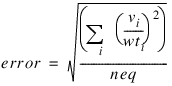
Norm_fcn—Name of a user-supplied procedure that estimates the error in each step. The parameter list is v, wt, error. v and wt are input as neq-element arrays, and error is a scalar output. By default:
All floating point input will be double precision and all output must be of type double precision.
User_jac_factor_solve—A 3-element array of names of procedures that compute pdg (see the Jacobian keyword), factor pdg, and solve pdgTdy = dg. User_jac_factor_solve(0) is the same as the Jacobian keyword except that pdg is not a parameter and must be put in a common block shared by all three procedures. User_jac_factor_solve(1) factors pdg or checks its condition number, and its only parameter is set to zero for success or nonzero for failure. The User_jac_factor_solve(2) parameter list is dg and dy, where dg is an input neq-element array, and the output dy is the solution to pdgTdy = dg. Defaults to internal computation. As with all the other user procedures, all floating point input will be double precision and all output must be of type double precision.
Atol_rtol_arrays—An (
neq,2) array.
Atol_rtol_arrays(
i,*) are the absolute and relative tolerances on
yi. By default, all tolerances are set to
. See the MACHINE function.
Max_numbersteps—Maximum number of steps that can be used to advance from t(i) to t(i+1). The default is 500.
Max_step—Maximum step size allowed. Default: unlimited.
All_nonnegative—If nonzero, the solver forces yi ≥ 0. By default, this constraint is not enforced.
Bdf_order_next_step—The order of the BDF method to use on all steps. By default, this is computed internally.
Output Keywords
Bdf_order_previous_step—The BDF order used on last step.
Nsteps_taken—The number of steps taken.
Nfcng—The number of times that g has been evaluated.
Nfcnj—The number of evaluations of pdg (see the Jacobian keyword).
Nerror_test_failures—The number of error test failures.
Nconv_test_failures—The number of convergence test failures.
Condition—The highest condition number attained by pdg(t). This option cannot be used if User_jac_factor_solve was used.
Description
DEA_PETZOLD_GEAR finds an approximation to the solution of a system of differential-algebraic equations g(t, y, y') = 0, with given initial data for y and y'. DEA_PETZOLD_GEAR uses BDF formulas, appropriate for systems of stiff ODEs, and attempts to keep the global error proportional to a user-specified tolerance. See Brenan et al. (1989). DEA_PETZOLD_GEAR is efficient for stiff differential-algebraic systems of index 1 or index 0. See Brenan et al. (1989) for a definition of index. DEA_PETZOLD_GEAR is based on the code DASSL designed by L. Petzold (1982-1990). DEA_PETZOLD_GEAR does all computations in double precision.
Example 1
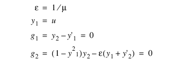
The Van der Pol equation u” + μ(u2 – 1) u' + u = 0, μ > 0, is a single ordinary differential equation with a periodic limit cycle. See Hartman (1964, page 181). For the value μ = 5, the equation is integrated from t = 0 until the limit has clearly developed at t = 26. The (arbitrary) initial conditions used here are u(0) = 2 and u'(0) = –2/3. Except for these initial conditions and the final t value, this is problem (E2) of the Enright and Pryce (1987) test package. This equation is solved as a differential-algebraic system by defining the first-order system:
Note that the initial condition for the sample program is not consistent, g ≠ 0 at t = 0. The Initial_values_inconsistent keyword is used to reflect this.
This example is available in <RW_DIR>/wave/lib/user/examples/dea_petzold_gear_exmp.pro.
PRO gcn1, t, y, ypr, gval, f
gval = [ y(1)-ypr(0), (1-y(0)*y(0))*y(1)-0.2*(y(0)+ypr(1)) ]
f = 0d
END
PRO dea_petzold_gear_ex1, nopl=nopl
t = DINDGEN(261) / 10
y = [ 2, -2/3d ]
ypr = [ y(1), 0 ]
DEA_PETZOLD_GEAR, "gcn1", t, y, ypr, $
/Initial_Values_Inconsistent
PM, [ ' ', 'Example 1 - Van der Pol equations' ]
PM, "y values at t=26:", y(*,260), Format='(a20,2e20.4)'
PM, "y' values at t=26:", ypr(*,260), Format='(a20,2e20.4)'
IF N_ELEMENTS(nopl) EQ 0 THEN BEGIN
titl = "Van der Pol Cycle, (u(t),u'(t)), mu=5"
posi = [ 0.06, 0.06, 0.94, 0.94 ]
WINDOW, Xsize=600, Ysize=600
PLOT, y(0,2:*), y(1,2:*), Psym=1, Title=titl, $
Position=posi, / Norm
ENDIF
END
Output
Example 1 - Van der Pol equations
y values at t=26: 1.4877e+000 -2.3200e-001
y' values at t=26: -2.3200e-001 -8.0291e-002
Example 2
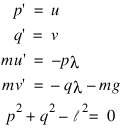
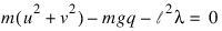
The first-order equations of motion of a point-mass m suspended on a massless wire of length l under the influence of gravity force, mg and tension value λ, in Cartesian coordinates, (p, q), are:
This is a genuine differential-algebraic system. The problem, as stated, has an index number equal to the value 3. Thus, it cannot be solved with DEA_PETZOLD_GEAR directly. Unfortunately, the fact that the index is greater than 1 must be deduced indirectly. Typically there will be an error processed which states that the (BDF) corrector equation did not converge. The user then differentiates and replaces the constraint equation. This example is transformed to a problem of index number of value 1 by differentiating the last equation twice. This resulting equation, which replaces the given equation, is the total energy balance:
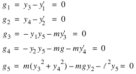
With initial conditions and systematic definitions of the dependent variables, the system becomes:
The problem is given in English measurement units of feet, pounds, and seconds. The wire has length 6.5 ft, and the mass at the end is 98 lb. Usage of the software does not require it, but standard or “SI” units are used in the numerical model. This conversion of units is done as a first step in the user-supplied evaluation function gcn. A set of initial conditions, corresponding to the pendulum starting in a horizontal position, are provided as output for the input signal of n = 0. The maximum magnitude of the tension parameter, λ(t) = y5(t), is computed at the output points, t = 0.1, π, 0.1. This extreme value is converted to English units and printed.
This example is available in <RW_DIR>/wave/lib/user/examples/dea_petzold_gear_exmp.pro.
PRO gcn2, t, y, ypr, gval, f
COMMON gcn2, masskg, mg, lensq
gval = DBLARR(5)
gval(0) = y(2) - ypr(0)
gval(1) = y(3) - ypr(1)
gval(2) = -y(0)*y(4) - masskg*ypr(2)
gval(3) = -y(1)*y(4) - masskg*ypr(3) - mg
gval(4) = masskg*(y(2)*y(2)+y(3)*y(3)) - mg*y(1) - lensq*y(4)
f = 0d
END
PRO dea_petzold_gear_ex2
COMMON gcn2, masskg, mg, lensq
meterl = 1.9812d
masskg = 44.4520531d
grav = 9.8066502d
mg = masskg * grav
lensq = meterl * meterl
t = DINDGEN(32) / 10
y = [ meterl, 0, 0, 0, 0 ]
ypr = [ 0d, 0, 0, 0, 0 ]
DEA_PETZOLD_GEAR, "gcn2", t, y, ypr
PM, [ ' ', 'Example 2 - First-order equations of motion' ]
PM, 'maximum tension', MAX(ABS(y(4,*)),imax)/0.4536, $
Format='(a20,e20.4)'
PM, 'angle at max tension', t(imax), Format='(a20,e20.4)'
END
Output
Example 2 - First-order equations of motion
maximum tension 1.4552e+003
angle at max tension 2.5000e+000
Example 3
In this example, we solve a stiff ordinary differential equation (E5) from the test package of Enright and Pryce (1987). The problem is nonlinear with nonreal eigenvalues. It is included as an example because it is a stiff problem, and its partial derivatives are provided in the user supplied function. Providing explicit formulas for partial derivatives is an important consideration for problems where evaluations of the function g(t, y, y') are expensive. In addition, an initial integration step-size is given for this test problem. The error tolerance is changed from the defaults to a pure absolute tolerance.
This example is available in <RW_DIR>/wave/lib/user/examples/dea_petzold_gear_exmp.pro.
PRO gcn3, t, y, ypr, gval, f
c1 = 7.89d-10
c2 = 1.1d7
c3 = 1.13d9
c4 = 1.13d3
gval = DBLARR(4)
gval(0) = -c1*y(0)-c2*y(0)*y(2)-ypr(0)
gval(1) = c1*y(0)-c3*y(1)*y(2)-ypr(1)
gval(2) = c1*y(0)-c2*y(0)*y(2)+c4*y(3)-c3*y(1)*y(2)-ypr(2)
gval(3) = c2*y(0)*y(2) - c4*y(3) - ypr(3)
f = 0d
END
PRO jgcn3, t, y, ypr, cj, pdg
c1 = 7.89d-10
c2 = 1.1d7
c3 = 1.13d9
c4 = 1.13d3
pdg(0,0) = -c1-c2*y(2)-cj
pdg(2,0) = -c2*y(0)
pdg(0,1) = c1
pdg(1,1) = -c3*y(2)-cj
pdg(2,1) = -c3*y(1)
pdg(0,2) = c1-c2*y(2)
pdg(1,2) = -c3*y(2)
pdg(2,2) = -c2*y(0)-c3*y(1)-cj
pdg(3,2) = c4
pdg(0,3) = c2*y(2)
pdg(2,3) = c2*y(0)
pdg(3,3) = -c4-cj
END
PRO dea_petzold_gear_ex3
t = [ 0d, 1000 ]
y = [ 1.76d-3, 0, 0, 0 ]
ypr = [ 0d, 0, 0, 0 ]
mach = MACHINE(/Float)
scalar_values = REBIN( [[0.1d*SQRT(mach.max_rel_space)], $
[0]], 4, 2 )
DEA_PETZOLD_GEAR, "gcn3", t, y, ypr, $
Initial_Stepsize=5.0d-5, Jacobian="jgcn3", $
Atol_Rtol_Arrays=scalar_values
PM, [ ' ', 'Example 3 - Stiff ODE from Enright & Pryce' ]
PM, "y at t=1000:", y(*,1), Format='(a16,4e16.4)'
PM, "y' at t=1000:", ypr(*,1), Format='(a16,4e16.4)'
END
Output
Example 3 - Stiff ODE from Enright & Pryce
y at t=1000: 1.6201e-003 1.3837e-010 8.2496e-012 1.3012e-010
y'at t=1000: -1.3830e-007 -1.1423e-014 -1.9098e-017 -1.1404e-014
Example 4
In this example, we compute the solution of n = 10 ordinary differential equations, g = Hy – y', where y(0) = y0 = (1, 1, ..., 1)T. The value:
is evaluated at t = 1. The constant matrix H has entries hi,j = min(j – i, 0) so it is lower Hessenberg. We use COMMON blocks to pass H to the user-supplied functions for the evaluation of the following intermediate quantities:
1. The function g.
2. The partial derivative matrix A = ∂g/∂y + cj∂g/∂y' = H – cjI.
This example is available in <RW_DIR>/wave/lib/user/examples/dea_petzold_gear_exmp.pro.
PRO gcn4, t, y, ypr, gval, f
COMMON gcn4, h, i
gval = h#y - ypr
f = 0d
END
PRO jgcn4, t, y, ypr, cj, pdg
COMMON gcn4, h, i
pdg(0,0) = h
pdg(i,i) = pdg(i,i) - cj
END
PRO dea_petzold_gear_ex4
COMMON gcn4, h, i
t = [ 0d, 1 ]
n = 10
y = REPLICATE(1d,n)
ypr = DBLARR(n)
i = LINDGEN(n)
h = TENSOR_SUB(-i,-i) < 0d
h(i(0:n-2),i(0:n-2)+1) = 1
DEA_PETZOLD_GEAR, "gcn4", t, y, ypr, Jacobian="jgcn4"
PM, [ ' ', 'Example 4 - 10 ODEs' ]
PM, "sum of y(i) at t=1:", TOTAL(y(*,1)), $
Format='(a20,e20.4)'
END
Output
Example 4 - 10 ODEs
sum of y(i) at t=1: 6.5186e+001
Example 5
In this example, we solve the same problem as in Example 4, but use the User_jac_factor_solve keyword to supply functions to compute the partial derivatives A = [∂g/∂y + cj∂g/∂y']', factor A, and solve the system AΔy = Δg. The problem specific data in this example is the lower Hessenberg matrix H, and the array A that will contain the partial derivatives A = [∂g/∂y + cj∂g/∂y']', and factored form of this matrix. Note, in this example, the matrix A containing the partial derivatives and factored form of this matrix is stored local to the example. Using the User_jac_factor_solve keyword allows us to apply problem specific techniques to factor A, and solve the system AΔy = Δg.
This example can also serve as a prototype for large, structured (possibly nonlinear) DAE problems where the user must use special methods to store and factor the matrix A and solve the linear system AΔy = Δg. The word “factor” is used liberally here. A user could, for instance, solve the system using an iterative method. Generally, the factor step can be any preparatory phase required for a later solve step.
This example is available in <RW_DIR>/wave/lib/user/examples/dea_petzold_gear_exmp.pro.
PRO gcn5, t, y, ypr, gval, f
COMMON gcn5, h, i, pdg
gval = h#y - ypr
f = 0d
END
PRO jgcn5, t, y, ypr, cj
COMMON gcn5, h, i, pdg
pdg(0,0) = h
pdg(i,i) = pdg(i,i) - cj
END
PRO fac5, err
COMMON gcn5, h, i, pdg
err = 0d
END
PRO sol5, dg, dy
COMMON gcn5, h, i, pdg
dy = INV(TRANSPOSE(pdg), /Double) # dg
END
PRO dea_petzold_gear_ex5
COMMON gcn5, h, i, pdg
t = [ 0d, 1 ]
n = 10
y = REPLICATE(1d,n)
ypr = DBLARR(n)
i = LINDGEN(n)
h = TENSOR_SUB(-i,-i) < 0d
h(i(0:n-2),i(0:n-2)+1) = 1
pdg = h
DEA_PETZOLD_GEAR, "gcn5", t, y, ypr, $
user_jac_factor_solve=["jgcn5","fac5","sol5"]
PM, [' ','Example 5 - Same as example 4, but with ' + $
'USER_JAC_FACTOR_SOLVE']
PM, "sum of y(i) at t=1:", TOTAL(y(*,1)), $
Format='(a20,e20.4)'
END
; Main routine runs five dea_petzold_gear examples.
PRO dea_petzold_gear_exmp, nopl=nopl
IF NOT OPTION_IS_LOADED('math') THEN MATH_INIT dea_petzold_gear_ex1, nopl=nopl
dea_petzold_gear_ex2
dea_petzold_gear_ex3
dea_petzold_gear_ex4
dea_petzold_gear_ex5
END
Output
Example 5 - Same as example 4, but with USER_JAC_FACTOR_SOLVE
sum of y(i) at t=1: 6.5186e+001
Version 2017.0
Copyright © 2017, Rogue Wave Software, Inc. All Rights Reserved.