LINEAR_PROGRAMMING Function (PV-WAVE Advantage)
Minimizes the Euclidean scalar product cTx on Rn, for fixed c, linear constraints bl ≤ Ax ≤ bu, and bounds xl ≤ x ≤ xu.
Usage
x = linear_programming(a, bl, bu, c)
Input Parameters
a—An (m,p) constraint matrix. Usually p=n=n_elements(x), but p<n can be used to limit the constraints to x(0:p–1).
bl—An m-element vector of lower bounds for the constraints. If the ith constraint is not bounded below then set bl(i) = –1e30 or use the Irtype keyword. For an equality, set bl(i) = bu(i), or use the Irtype keyword.
bu—An m-element vector of upper bounds for the constraints. If the ith constraint is not bounded above then set bu(i) = 1e30 or use the Irtype keyword. For an equality, set bl(i)=bu(i), or use the Irtype keyword.
c—An n-element vector defining the objective function.
Returned Value
x—The n-element solution vector.
Input Keywords
Xl—An n-element vector of lower bounds for the solution x. If x(i) is unbounded below, set Xl(i) = –1e30. Default: Xl(*)=0.
Xu—An n-element vector of upper bounds for the solution x. If x(i) is unbounded above, set Xu(i) = 1e30. Default: Xu(*)=1e30.
File—A 4-element string array. If supplied, the a, bl, bu, c, Xl, and Xu inputs are ignored and instead extracted from the mps file file(0). file(1:3) are respectively the names of the RHS set, the Ranges set, and the Bounds set to be used. If the name is the null string '', then the first set in the file is used. See the MPS File section.
Irtype—An m-element vector of positive integers which can be used to override the constraint bounds bl ≤ Ax ≡ r ≤ bu.
 irtype
(
i) = 0 imposes the equality
bl(
i) =
r(
i)
irtype(
i) = 1 imposes the inequality
r(
i)
≤ bu(
i)
irtype(
i) = 2 imposes the inequality
bl(
i)
≤ r(
i)
irtype(
i) = 3 imposes the inequality
bl(
i)
≤ r(
i)
≤ bu(
i)
irtype(
i) = 4 disables the
ith constraint
Defaults to irtype(*)=3
Refinement—If set, the solution is checked for consistency and if necessary, refined for more accuracy. Default: not set.
Extended_refinement—If set, refinement (see above) is repeated iteratively for maximum possible accuracy. Default: not set.
Output Keywords
Obj—The optimal value of the objective function.
Niter—The number of iterations.
Dual—An m-element vector containing the dual solution. Dual must be a named variable on input.
Description
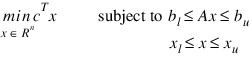
LINEAR_PROGRAMMING uses an active set strategy to solve linear programming problems, i.e., problems of the form:
where c is the objective coefficient vector, A is the coefficient matrix, and the vectors bl, bu, xl, and xu are the lower and upper bounds on the constraints and the variables, respectively.
If the Refinement keyword is used, the coefficient matrices and other data are saved at the beginning of the computation. When finished this data together with the solution obtained is checked for consistency. If the discrepancy is too large, the solution process is restarted using the problem data just after processing the equalities, but with the final x values and final active set. By default refinement is not performed.
If the Extended_refinement keyword is used, refinement is performed iteratively until there is a sign that no further progress is possible (recommended if all the accuracy possible is desired). By default extended refinement is not performed.
Refer to the following paper for further information: Krogh, Fred, T. (2005),
An Algorithm for Linear Programming,
http://mathalacarte.com/fkrogh/pub/lp.pdf , Tujunga, CA.
MPS File Format
There is some variability in the MPS format. This section describes the MPS format accepted by LINEAR_PROGRAMMING.
An MPS file consists of a number of sections. Each section begins with a name in column 1. With the exception of the NAME section, the rest of this line is ignored. Lines with a ‘*’ or ‘$’ in column 1 are considered comment lines and are ignored.
The body of each section consists of lines divided into fields, as follows:
The format limits MPS names to 8 characters and values to 12 characters. The names in fields 2, 3, and 5 are case sensitive. Leading and trailing blanks are ignored, but internal spaces are significant.
The sections in an MPS file are as follows:
NAME
ROWS
COLUMNS
RHS
RANGES (optional)
BOUNDS (optional)
QUADRATIC (optional)
ENDATA
Sections must occur in the above order.
MPS keywords (defined by the user in MPS data files), section names and indicator values, are case insensitive. Row, column and set names are case sensitive.
NAME Section
The NAME section contains the single line. A problem name can occur anywhere on the line after NAME and before columns 62. The problem name is truncated to 8 characters.
ROWS Section
The ROWS section defines the name and type for each row. Field 1 contains the row type and field 2 contains the row name. Row type values are not case sensitive. Row names are case sensitive. The following row types are allowed:
E—Equality Constraint.
L—Less than or equal constraint.
G—Greater than or equal constraint.
N—Objective or a free row.
COLUMNS Section
The COLUMNS section defines the nonzero entries in the objective and the constraint matrix. The row names here must have been defined in the ROWS section.
2—Column name.
3—Row name.
4—Value for the entry whose row and column are given by fields.
5—Row name.
6—Value for entry whose row and column are given by fields 5 and 2.
note | Fields 5 and 6 are optional. |
The COLUMNS section can also contain markers. These are indicated by the name ‘MARKER’ (with the quotes) in field 3 and the marker type in field 4 or 5.
Marker type ‘INTORG’ (with the quotes) begins an integer group. The marker type ‘INTEND’ (with the quotes) ends this group. The variables corresponding to the columns defined within this group are required to be integers.
RHS Section
The RHS section defines the right-hand side of the constraints. An MPS file can contain more than one RHS set, distinguished by the RHS set name. The row names here must be defined in the ROWS section.
2—RHS set name.
3—Row name.
4—Value for the entry whose set and row are given by fields 2 and 3.
5—Row name.
6—Value for the entry whose set and row are given by fields 2 and 5.
note | Fields 5 and 6 are optional. |
RANGES Section
The optional RANGES section defines two-sided constraints. An MPS file can contain more than one range set, distinguished by the range set name. The row names here must have been defined in the ROWS section.
2—Range set name.
3—Row name.
4—Value for the entry whose set and row are given by fields 2 and 3.
5—Row name.
6—Value for the entry whose set and row are given by fields 2 and 5.
note | Fields 5 and 6 are optional. |
Ranges change one-sided constraints, defined in the RHS section, into two-sided constraints. The two-sided constraint for row
i depends on the range value,
ri, defined in this section. The right-hand side value,
bi, is defined in the RHS section. The two-sided constraints for row
i are given in
Range Constraints:
BOUNDS Section
The optional BOUNDS section defines bounds on the variables. By default, the bounds are 0 ≤ xi ≤ ∞. The bounds can also be used to indicate that a variable must be an integer.
More than one bound can be set for a single variable. For example, to set 2 ≤ xi ≤ 6 use a LO bound with value 2 to set 2 ≤ xi and an UP bound with value 6 to add the condition xi ≤ 6.
An MPS file can contain more than one bounds set, distinguished by the bound set name.
1—Bounds type.
2—Bounds set name.
3—Column name
4—Value for the entry whose set and column are given by fields 2 and 3.
5—Column name.
6—Value for the entry whose set and column are given by fields 2 and 5.
note | Fields 5 and 6 are optional. |
The bound types are as follows. Here bi are the bound values defined in this section, the xi are the variables, and I is the set of integers.
The bound type names are not case sensitive. If the bound type is UP or UI and bj < 0 then the lower bound is set to –∞.
QUADRATIC Section
The optional QUADRATIC section defines the Hessian for quadratic programming problems. The names HESSIAN, QUADS, QUADOBJ, QSECTION and QMATRIX are also recognized as beginning the QUADRATIC section.
2—Column name.
3—Column name
4—Value for entry whose row and column are given by fields 2 and 3.
5—Column name.
6—Value for entry whose row and column are given by fields 2 and 4.
note | Fields 5 and 6 are optional. |
ENDATA Section
The ENDATA section ends the MPS file.
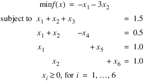
Example 1
The linear programming problem in the standard form:
is solved.
This example is available in <RW_DIR>/wave/lib/user/examples/linear_programming_ex.pro.
MATH_INIT
a = [ [1,1,1,0],[1,1,0,1],[1,0,0,0],[0,-1,0,0],[0,0,1,0], $
[0,0,0,1] ]
b = [ 1.5, 0.5, 1.0, 1.0 ]
c = [ -1, -3, 0, 0, 0, 0 ]
x = LINEAR_PROGRAMMING(a,b,b,c)
Output
Running this example from<RW_DIR>/wave/lib/user/examples/linear_programming_ex.pro produces the following:
x =
0.500 1.000 0.000 1.000 0.500 0.000
Example 2
This example demonstrates how the
file keyword can be used with LINEAR_PROGRAMMING to solve a linear programming problem defined in an MPS file. The MPS file used in this example is an
uncompressed version of the file ‘afiro’, available from
http://www.netlib.org/lp/data/. This example also demonstrates the use of the
refinement keyword to activate iterative refinement.
This example is available in <RW_DIR>/wave/lib/user/examples/linear_programming_ex.pro.
MATH_INIT
file = [ GETENV('WAVE_DIR')+'/lib/user/examples/afiro', $ '', '', '' ]
x = LINEAR_PROGRAMMING( File=file, /Refinement, Obj=obj )
Output
Running this example from<RW_DIR>/wave/lib/user/examples/linear_programming_ex.pro produces the following:
x =
80.0 25.5 54.5 84.8 57.9 0.0 0.0 0.0
0.0 0.0 0.0 0.0 18.2 39.7 61.3 500.0
475.9 24.1 0.0 215.0 363.9 0.0 0.0 0.0
0.0 0.0 0.0 0.0 339.9 20.1 156.5 0.0
obj =
-464.753
Errors
MULTIPLE_SOLUTIONS—Multiple solutions giving essentially the same minimum exist.
Warning Errors
SOME_CONSTRAINTS_DISCARDED—Some constraints were discarded because they were too linearly dependent on other active constraints.
ALL_CONSTR_NOT_SATISFIED—All constraints are not satisfied. If a feasible solution is possible then try using refinement by supplying the Refinement keyword.
CYCLING_OCCURRING—The algorithm appears to be cycling. Using refinement may help.
Fatal Errors
PROB_UNBOUNDED—The problem is unbounded.
PIVOT_NOT_FOUND—An acceptable pivot could not be found.
Version 2017.0
Copyright © 2017, Rogue Wave Software, Inc. All Rights Reserved.