model—Four element array containing the numbers p, q, s, d of the ARIMA  , model the outlier free series is following.
, model the outlier free series is following., model the outlier free series is following. :
:
 , can be computed as:
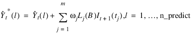
 is done in two steps:
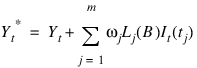
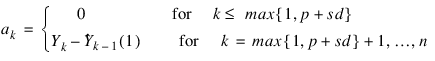
 , can be computed recursively as:
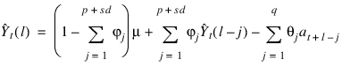
 by adding the multiple outlier effects to the forecasts for {Yt}.
Outlier | Formula |
Innovational outliers (IO) | 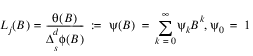 |
Additive outliers (AO) | Lj(B) = 1 |
Level shifts (LS) | 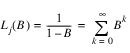 |
Temporary changes (TC) | 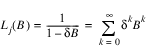 |
Outlier | Formula |
Innovational outliers (IO) |  |
Additive outliers (AO) |  |
Level shifts (LS) | 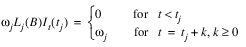 |
Temporary changes (TC) | 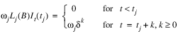 |
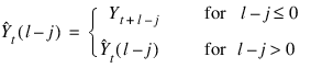
 can be computed easily.
 and Yt+1 are given by:
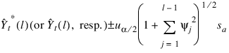
 is the 100(1 – α/2) percentile of the standard normal distribution,
  is an estimate of the variance
  of the random shocks (returned from TS_OUTLIER_IDENTIFICATION), and the ψ weights {ψj} are the coefficients in:
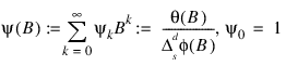
time_series = [ $
41.67 , 41.67 , 42.0752144, 42.6123962, $
43.6161919, 42.1932831, 43.1055450, 44.3518715, $
45.3961258, 45.0790215, 41.8874397, 40.2159805, $
40.2447319, 39.6208458, 38.6873589, 37.9272423, $
36.8718872, 36.8310852, 37.4524879, 37.3440933, $
37.9861374, 40.3810501, 41.3464622, 42.6495285, $
42.6096764, 40.3134537, 39.7971268, 41.5401535, $
40.7160759, 41.0363541, 41.8171883, 42.4190292, $
43.0318832, 43.9968109, 44.0419617, 44.3225212, $
44.6082611, 43.2199631, 42.0419197, 41.9679718, $
42.4926224, 43.2091255, 43.2512283, 41.2301674, $
40.1057358, 40.4510574, 41.5329170, 41.5678177, $
43.0090141, 42.1592140, 39.9234505, 38.8394127, $
40.4319878, 40.8679352, 41.4551926, 41.9756317, $
43.9878922, 46.5736389, 45.5939293, 42.4487762, $
41.5325394, 42.8830910, 44.5771217, 45.8541985, $
46.8249474, 47.5686378, 46.6700745, 45.4120026, $
43.2305107, 42.7635345, 43.7112923, 42.0768661, $
41.1835632, 40.3352280, 37.9761467, 35.9550056, $
36.3212509, 36.9925880, 37.2625008, 37.0040665, $
38.5232544, 39.4119797, 41.8316803, 43.7091446, $
42.9381447, 42.1066780, 40.3771248, 38.6518707, $
37.0550499, 36.9447708, 38.1017685, 39.4727097, $
39.8670387, 39.3820763, 38.2180786, 37.7543488, $
37.7265244, 38.0290642, 37.5531158, 37.4685936, $
39.8233147, 42.0480766, 42.4053535, 43.0117416, $
44.1289330, 45.0393829, 45.1114540, 45.0086479, $
44.6560631, 45.0278931, 46.7830849, 48.7649765, $
47.7991905, 46.5339661, 43.3679199, 41.6420822, $
41.2694893, 41.5959740, 43.5330009, 43.3643608, $
42.1471291, 42.5552788, 42.4521446, 41.7629128, $
39.9476891, 38.3217010, 40.5318718, 42.8811569, $
44.4796944, 44.6887932, 43.1670265, 41.2226143, $
41.8330154, 44.3721924, 45.2697029, 44.4174194, $
43.5068550, 44.9793015, 45.0585403, 43.2746620, $
40.3317070, 40.3880501, 40.2627106, 39.6230278, $
41.0305252, 40.9262009, 40.8326912, 41.7084885, $
42.9038048, 45.8650513, 46.5231590, 47.9916115, $
47.8463135, 46.5921936, 45.8854408, 45.9130440, $
45.7450371, 46.2964249, 44.9394569, 45.8141251, $
47.5284042, 48.5527802, 48.3950577, 47.8753052, $
45.8880005, 45.7086983, 44.6174774, 43.5567932, $
44.5891113, 43.1778679, 40.9405632, 40.6206894, $
41.3330421, 42.2759552, 42.4744949, 43.0719833, $
44.2178459, 43.8956337, 44.1033440, 45.6241455, $
45.3724861, 44.9167595, 45.9180603, 46.9077835, $
46.1666603, 46.6013489, 46.6592331, 46.7291603, $
47.1908340, 45.9784355, 45.1215782, 45.6791115, $
46.7379875, 47.3036957, 45.9968834, 44.4669495, $
45.7734680, 44.6315041, 42.9911766, 46.3842583, $
43.7214432, 43.5276833, 41.3946495, 39.7013168, $
39.1033401, 38.5292892, 41.0096245, 43.4535828, $
44.6525154, 45.5725899, 46.2815285, 45.2766647, $
45.3481712, 45.5039482, 45.6745682, 44.0144806, $
42.9305000, 43.6785469, 42.2500534, 40.0007210, $
40.4477005, 41.4432716, 42.0058670, 42.9357758, $
45.6758842, 46.8809929, 46.8601494, 47.0449791, $
46.5420647, 46.8939934, 46.2963371, 43.5479164, $
41.3864059, 41.4046364, 42.3037987, 43.6223717, $
45.8602371, 47.3016396, 46.8632469, 45.4651413, $
45.6275482, 44.9968376, 42.7558670, 42.0218239, $
41.9883728, 42.2571678, 44.3708687, 45.7483635, $
44.8832512, 44.7945862, 44.8922577, 44.7409401, $
45.1726494, 45.5686874, 45.9946709, 47.3151054, $
48.0654068, 46.4817467, 42.8618279, 42.4550323, $
42.5791168, 43.4230957, 44.7787971, 43.8317108, $
43.6481781, 42.4183960, 41.8426285, 43.3475227, $
44.4749908, 46.3498306, 47.8599319, 46.2449913, $
43.6044006, 42.4563484, 41.2715340, 39.8492508, $
39.9997292, 41.4410820, 42.9388237, 42.5687332]
; We will use the first 280 to generate a forecast for the
; next 10 and test that forecast against these 10 actual
; observations.
forecast_actual = [42.6384087, 41.7088661, 43.9399033, $
45.4284401, 44.4558411, 45.1761856, $
45.3489113, 45.1892662, 46.3754730, $
45.6082802]
delta = 0.7
n_predict = 10
model = [2, 1, 1, 0]
result = TS_OUTLIER_IDENTIFICATION( $
model, time_series, $
Relative_Error=1.0e-4, $
Num_Outliers=num_outliers, $
Residual=residual, $
Outlier_Statistics=outlier_stat, $
Omega_Weights=omega, $
Arma_Param=parameters, $
Res_Sigma=res_sigma, $
Aic=aic)
PRINT, "ARMA parameters:"
PRINT, parameters, Format='(F11.6)'
PRINT, ''
PRINT, num_outliers, Format="('Number of outliers: ', I1)"PRINT, ''
PRINT, "Outlier statistics:"
PRINT, "Time point Outlier type"
FOR i=0L, num_outliers-1 DO $
PRINT, outlier_stat(i,0), outlier_stat(i,1), $
Format="(I6, 10X, I3)"
PRINT, ''
PRINT, res_sigma, Format="('RSE: ', F11.6)"PRINT, aic, Format="('AIC: ', F11.6)"PRINT, ''
; collect the output from the TS_OUTLIER_IDENTIFICATION call
; and arrange it for the call to TS_OUTLIER_FORECAST
series = FLTARR(N_ELEMENTS(time_series),2)
series(*,0) = time_series
series(*,1) = residual
forecast = TS_OUTLIER_FORECAST( $
series, $
outlier_stat, omega, delta, $
model, parameters, n_predict, $
Out_Free_Forecast=outfree_forecast)
forecast_table = FLTARR(n_predict,4)
PRINT, "** " + $
"Forecast Table for Outlier Contaminated Series **"
PRINT, "Orig. Series Forecast Prob. Limits PSI Weights"
FOR i=0L, n_predict-1 DO $
PRINT, forecast_actual(i), forecast(i,0), $
forecast(i,1), forecast(i,2), $
Format='(F10.4, 3F13.4)'
PRINT, ''
PRINT, "****** " + $
"Forecast Table for Outlier Free Series ******"
PRINT, " Outlier"
PRINT, " Free Series Forecast Prob. Limits PSI Weights"
FOR i=0L, n_predict-1 DO BEGIN & $
PRINT, forecast_actual(i), outfree_forecast(i,0), $
outfree_forecast(i,1), outfree_forecast(i,2), $
Format='(F10.4, 3F13.4)' & $
ENDFOR
ARMA parameters:
8.891920
0.944060
-0.150423
-0.558918
Number of outliers: 2
Outlier statistics:
Time point Outlier type
150 2
200 1
RSE: 1.004306
AIC: 1323.617554
** Forecast Table for Outlier Contaminated Series **
Orig. Series Forecast Prob. Limits PSI Weights
42.6384 43.6852 1.9684 1.5030
41.7089 43.8266 3.5535 1.2685
43.9399 44.0516 4.3430 0.9714
45.4284 44.2428 4.7453 0.7263
44.4558 44.3895 4.9560 0.5395
45.1762 44.4992 5.0685 0.4001
45.3489 44.5807 5.1293 0.2966
45.1893 44.6411 5.1624 0.2198
46.3755 44.6859 5.1805 0.1629
45.6083 44.7191 5.1904 0.1207
****** Forecast Table for Outlier Free Series ******
Outlier
Free Series Forecast Prob. Limits PSI Weights
40.1384 41.9598 1.9684 1.5030
39.2089 42.1012 3.5535 1.2685
41.4399 42.3262 4.3430 0.9714
42.9284 42.5174 4.7453 0.7263
41.9558 42.6641 4.9560 0.5395
42.6762 42.7738 5.0685 0.4001
42.8489 42.8553 5.1293 0.2966
42.6893 42.9157 5.1624 0.2198
43.8755 42.9605 5.1805 0.1629
43.1083 42.9937 5.1904 0.1207