AUTO_ARIMA Function (PV-WAVE Advantage)
Automatically identifies time series outliers, determines parameters of a multiplicative seasonal ARIMA

model and produces forecasts that incorporate the effects of outliers whose effects persist beyond the end of the series.
Usage
result = AUTO_ARIMA (tpoints, x)
Input Parameters
tpoints—Array of length n_obs containing the time points t1, t2, ..., tn_obs the time series was observed, where n_obs is the number of observations in the original time series. It is required that t1, t2, ..., tn_obs are in strictly ascending order.
x—Array of length
n_obs containing the observed time series values
. This can contain outliers and missing observations. Outliers are identified by this routine and missing values are identified by the time values in
tpoints. If the time interval between two consecutive time points is greater than one, i.e.,
ti+1 –
ti =
m > 1, then
m – 1 missing values are assumed to exist between
ti and
ti+1 at times
ti + 1,
ti + 2,
...,
ti+1 – 1. Therefore, the gap free series is assumed to be defined for equidistant time points
t1,
ti + 1, ...,
tn_obs. Missing values are automatically estimated prior to identifying outliers and producing forecasts. Forecasts are generated for both missing and observed values.
Returned Value
result—Array of length 1 +
p +
q with the estimated constant, AR and MA parameters used to fit the outlier-free series using an ARIMA

model. Upon completion, if
d =
model(3) = 0, then an ARMA(
p,
q) model or AR(
p) model is fitted to the outlier-free version of the observed series

. If
d =
model(3) > 0, these parameters are computed for an ARMA(
p,
q) representation of the seasonally adjusted series
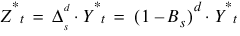
, where
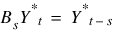
and
s =
model(2)
≥ 1.
Input Keywords
Double—If present and nonzero, double precision is used.
Method—The method used in model selection:

1—Automatic ARIMA

selection.
2—Grid search (Requires keywords
P_initial and
Q_initial.)
3—Specified ARIMA

model (
Model keyword required.)
Default: Method = 1
Maxlag—The maximum lag allowed when fitting an AR(p) model. Default: Maxlag = 10
Delta—The dampening effect parameter used in the detection of a Temporary Change Outlier (TC), 0 < Delta < 1. Default: Delta = 0.7
Critical—Critical value used as a threshold for outlier detection, Critical > 0. Default: Critical = 3.0
Epsilon—Positive tolerance value controlling the accuracy of parameter estimates during outlier detection. Default: Epsilon = 0.001
P_initial—A 1D integer array with N_p_initial elements containing the candidate values for p, from which the optimum is being selected. All candidate values in P_initial must be non-negative and N_p_initial ≥ 1. If Method = 2, then P_initial must be defined. Otherwise, P_initial is ignored.
Q_initial—A 1D integer array with N_q_initial elements containing the candidate values for q, from which the optimum is being selected. All candidate values in Q_initial must be non-negative and N_q_initial ≥ 1. If Method = 2, then Q_initial must be defined. Otherwise, Q_initial is ignored.
S_initial—A 1D integer array with N_s_initial elements containing the candidate values for s, from which the optimum is being selected. All candidate values in S_initial must be positive and N_s_initial ≥ 1. Default: S_initial = [1].
D_initial—A 1D integer array with N_d_initial elements containing the candidate values for d, from which the optimum is being selected. All candidate values in D_initial must be non-negative and N_d_initial ≥ 1. Default: D_initial = [0].
Num_predict—Number of forecasts requested. Forecasts are made at origin tn_obs, i.e. from the last observed value of the series. Default: Num_predict = 0.
Confidence—Confidence level for computing forecast confidence limits, taken from the exclusive interval (0, 100). Typical choices for Confidence are 90.0, 95.0, and 99.0. Default: Confidence = 95.0
Output Keywords
Model—(Input/Output) Array of length 4 containing the values for p, q, s, d. If Method=3 is chosen, then the values for p and q must be defined. If S_initial and D_initial are not defined, then s and d must also be given. If Method = 1 or Method = 2, then Model is ignored as an input array. On output, Model contains the optimum values for p, q, s, d in Model(0), Model(1), Model(2) and Model(3), respectively.
Residual—Array of length
n =
tn_obs –
t1 + 1
≥ n_obs, containing

, the estimates of the white noise in the outlier free original series.
Res_sigma—Residual standard error (RSE) of the outlier free original series.
Num_outliers—The number of outliers detected.
Outlier_statistics—A 2D array of size Num_outliers * 2 containing outlier statistics. The first column contains the time at which the outlier was observed (t = t1, t1 + 1, t1 + 2, ..., tn_obs) and the second column contains an identifier indicating the type of outlier observed. Outlier types fall into one of five categories:
0—Innovational Outliers (IO)
1—Additive Outliers (AO)
2—Level Shift Outliers (LS)
3—Temporary Change Outliers (TC)
4—Unable to Identify (UI)
If Num_outliers = 0, –1 is returned.
Aic—Akaike’s information criterion (AIC) for the optimum model.
Out_free_series—A 2D array of size
n by 2, where
n =
tn_obs –
t1 + 1. The first column of
Out_free_series contains the
n_obs observations from the original series,

, plus estimated values for any time gaps. The second column contains the same values as the first column adjusted by removing any outlier effects. In effect, the second column contains estimates of the underlying outlier-free series,
Yt. If no outliers are detected then both columns will contain identical values.
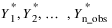
Out_free_forecast—A 2D array of size Num_predict by 3. The first column contains the forecasted values for the original outlier free series for t = tn_obs + 1, tn_obs + 2, ..., tn_obs + Num_predict. The second column contains standard errors for these forecasts, and the third column contains the psi weights of the infinite order moving average form of the model.
Outlier_forecast—A 2D array of size Num_predict by 3. The first column contains the forecasted values for the original series for t = tn_obs + 1, tn_obs + 2, ..., tn_obs + Num_predict. The second column contains standard errors for these forecasts, and the third column contains the ψ weights of the infinite order moving average form of the model.
Discussion
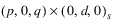
AUTO_ARIMA determines the parameters of a multiplicative seasonal ARIMA

model, and then uses the fitted model to identify outliers and prepare forecasts. The order of this model can be specified or automatically determined. The ARIMA

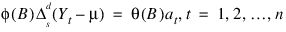
model handled by AUTO_ARIMA has the following form:
where:
and:
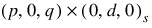
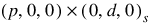
It is assumed that all roots of φ(B) and θ(B) lie outside the unit circle. Clearly, if s = 1 this reduces to the traditional ARIMA(p, d, q) model.
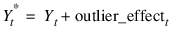
Yt is the unobserved, outlier-free time series with mean μ, and white noise at. This model is referred to as the underlying, outlier-free model. Function AUTO_ARIMA does not assume that this series is observable. It assumes that the observed values might be contaminated by one or more outliers, whose effects are added to the underlying outlier-free series:
Outlier identification uses the algorithm developed by Chen and Liu (1993). Outliers are classified into one of five types:
0—Innovational
1—Additive
2—Level Shift
3—Temporary Change
4—Unable to Identify
Once outliers are identified, AUTO_ARIMA estimates Yt, the outlier-free series representation of the data, by removing the estimated outlier effects.
Using the information about the adjusted ARIMA
model and the removed outliers, forecasts are then prepared for the outlier-free series. Outlier effects are added to these forecasts to produce a forecast for the observed series,

. If there are no outliers, then the forecasts for the outlier-free series and the observed series will be identical.
Model Selection
Users have an option of either supplying specific values for p, q, s, and d or have AUTO_ARIMA automatically select best fit values. Model selection can be conducted in one of three methods listed below depending upon the value of the Method keyword.
Method 1: Automatic ARIMA

Selection
This method initially searches for the AR(p) representation with minimum AIC for the noisy data, where p = 0, ..., Maxlag.
If
D_initial is defined then the values in
S_initial and
D_initial are included in the search to find an optimum ARIMA

representation of the series. Here, every possible combination of values for
p, s in
S_initial and
d in
D_initial is examined. The best found ARIMA
representation is then used as input for the outlier detection routine.
The optimum values for p, q, s, and d are returned in Model(0), Model(1), Model(2) and Model(3), respectively.
Method 2: Grid Search
The second automatic method conducts a grid search for p and q using all possible combinations of candidate values in P_initial and Q_initial. Therefore, for this method the P_initial and Q_initial keywords are required.
If the D_initial keyword is provided, the grid search is extended to include the candidate values for s and d given in S_initial and D_initial, respectively.
If the D_initial keyword is not used, no seasonal adjustment is attempted, and the grid search is restricted to searching for optimum values of p and q only.
The optimum values of p, q, s and d are returned in Model(0), Model(1), Model(2), and Model(3), respectively.
Method 3: Specified ARIMA

Model
In the third method, specific values for p, q, s and d are given. The values for p and q must be defined in model(0) and model(1), respectively. If the D_initial keyword is not used, then values s > 0 and d ≥ 0 must be specified in model(2) and model(3). If the D_initial keyword is provided, then a grid search for the optimum values of s and d is conducted using all possible combinations of input values in S_initial and D_initial. The optimum values of s and d can be found in model(2) and model(3), respectively.
note | Providing S_initial without D_initial causes a default value of 0 to be used for D_initial. In this case, no differencing is performed on the original time series. |
Outliers
The algorithm of Chen and Liu (1993) is used to identify outliers. The number of outliers identified is returned in
num_outliers. Both the time and classification for these outliers are returned in
outlier_statistics. Outliers are classified into one of five categories based upon the standardized statistic for each outlier type. The time at which the outlier occurred is given in the first column of
outlier_statistics. The outlier identifier returned in the second column is according to the descriptions in
Outlier Identifiers.
Except for additive outliers (AO), the effect of an outlier persists to observations following that outlier. Forecasts produced by AUTO_ARIMA take this into account.
Example 1
This example uses time series LNU03327709 from the US Department of Labor, Bureau of Labor Statistics. It contains the unadjusted special unemployment rate, taken monthly from January 1994 through September 2005. The values 01/2004 – 03/2005 are used by AUTO_ARIMA for outlier detection and parameter estimation. In this example, Method 1 without seasonal adjustment is chosen to find an appropriate AR(p) model. A forecast is done for the following six months and compared with the actual values 04/2005 – 09/2005.
model = INTARR(4)
x = [12.8, 12.2, 11.9, 10.9, 10.6, 11.3, 11.1, 10.4, 10.0, $
9.7, 9.7, 9.7, 11.1, 10.5, 10.3, 9.8, 9.8, 10.4, $
10.4, 10.0, 9.7, 9.3, 9.6, 9.7, 10.8, 10.7, 10.3, $
9.7, 9.5, 10.0, 10.0, 9.3, 9.0, 8.8, 8.9, 9.2, $
10.4, 10.0, 9.6, 9.0, 8.5, 9.2, 9.0, 8.6, 8.3, $
7.9, 8.0, 8.2, 9.3, 8.9, 8.9, 7.7, 7.6, 8.4, $
8.5, 7.8, 7.6, 7.3, 7.2, 7.3, 8.5, 8.2, 7.9, $
7.4, 7.1, 7.9, 7.7, 7.2, 7.0, 6.7, 6.8, 6.9, $
7.8, 7.6, 7.4, 6.6, 6.8, 7.2, 7.2, 7.0, 6.6, $
6.3, 6.8, 6.7, 8.1, 7.9, 7.6, 7.1, 7.2, 8.2, $
8.1, 8.1, 8.2, 8.7, 9.0, 9.3, 10.5, 10.1, 9.9, $
9.4, 9.2, 9.8, 9.9, 9.5, 9.0, 9.0, 9.4, 9.6, $
11.0, 10.8, 10.4, 9.8, 9.7, 10.6, 10.5, 10.0, 9.8, $
9.5, 9.7, 9.6, 10.9, 10.3, 10.4, 9.3, 9.3, 9.8, $
9.8, 9.3, 8.9, 9.1, 9.1, 9.1, 10.2, 9.9, 9.4, $
8.7, 8.6, 9.3, 9.1, 8.8, 8.5]
times = INDGEN(141) + 1
n_predict = 6
n_obs = 135
x_tmp = x(0:n_obs-1)
times_tmp = times(0:n_obs-1)
parameters = AUTO_ARIMA(times_tmp, x_tmp, $
Model=model, $
Aic=aic, $
Maxlag=5, $
Critical=4.0, $
Num_Outliers=num_outliers, $
Outlier_Statistics=outlier_stat, $
Res_Sigma=res_sigma, $
Num_Predict=n_predict, $
Outlier_Forecast=outlier_forecast)
PRINT, $
"Method 1: Automatic ARIMA model selection, no differencing"
PRINT, ''
PRINT, model(0), model(1), model(2), model(3), $
Format='("Model chosen: ", "p=", I1, ", q=", I1, ", ' + $ 's=", I1, ", d=", I1)'
PRINT, ''
PRINT, num_outliers, Format="('Number of outliers: ', I1)"PRINT, ''
PRINT, "Outlier statistics:"
PRINT, ''
PRINT, "Time point Outlier type"
FOR i=0L, num_outliers-1 DO $
PRINT, outlier_stat(i,0), outlier_stat(i,1), $
Format="(I6, 10X, I3)"
PRINT, ''
PRINT, res_sigma, Format="('RSE: ', F11.6)"PRINT, aic, Format="('AIC: ', F11.6)"PRINT, ''
p = model(0) + model(1)
PRINT, "Parameters:"
PRINT, parameters(0:(p)), Format='(F11.6)'
PRINT, ''
PRINT, " ** Forecast Table **"
PRINT, "Orig. Series Forecast Prob. Limits PSI Weights"
FOR i=0L, n_predict-1 DO $
PRINT, x(n_obs+i), outlier_forecast(i,0), $
outlier_forecast(i,1), outlier_forecast(i,2), $
Format='(F10.4, 3F13.4)'
Output
Method 1: Automatic ARIMA model selection, no differencing
Model chosen: p=5, q=0, s=1, d=0
Number of outliers: 2
Outlier statistics:
Time point Outlier type
97 0
109 0
RSE: 0.428036
AIC: 418.118958
Parameters:
0.166740
0.857958
-0.048228
-0.239798
0.200457
0.211682
** Forecast Table **
Orig. Series Forecast Prob. Limits PSI Weights
8.7000 9.0586 0.8389 0.8580
8.6000 9.0823 1.1054 0.6879
9.3000 9.4116 1.2470 0.3090
9.1000 9.6112 1.2736 0.2266
8.8000 9.5866 1.2877 0.3983
8.5000 9.4094 1.3304 0.5762
Example 2
This is the same as Example 1, except now AUTO_ARIMA uses Method 2 with a possible seasonal adjustment. As a result, the unadjusted model with p = 3, q = 2, s = 1, d = 0 is chosen as optimum.
model = INTARR(4)
s_initial = [1, 2]
d_initial = [0, 1, 2]
p_initial = [0, 1, 2, 3]
q_initial = [0, 1, 2, 3]
x = [12.8, 12.2, 11.9, 10.9, 10.6, 11.3, 11.1, 10.4, 10.0, $
9.7, 9.7, 9.7, 11.1, 10.5, 10.3, 9.8, 9.8, 10.4, $
10.4, 10.0, 9.7, 9.3, 9.6, 9.7, 10.8, 10.7, 10.3, $
9.7, 9.5, 10.0, 10.0, 9.3, 9.0, 8.8, 8.9, 9.2, $
10.4, 10.0, 9.6, 9.0, 8.5, 9.2, 9.0, 8.6, 8.3, $
7.9, 8.0, 8.2, 9.3, 8.9, 8.9, 7.7, 7.6, 8.4, $
8.5, 7.8, 7.6, 7.3, 7.2, 7.3, 8.5, 8.2, 7.9, $
7.4, 7.1, 7.9, 7.7, 7.2, 7.0, 6.7, 6.8, 6.9, $
7.8, 7.6, 7.4, 6.6, 6.8, 7.2, 7.2, 7.0, 6.6, $
6.3, 6.8, 6.7, 8.1, 7.9, 7.6, 7.1, 7.2, 8.2, $
8.1, 8.1, 8.2, 8.7, 9.0, 9.3, 10.5, 10.1, 9.9, $
9.4, 9.2, 9.8, 9.9, 9.5, 9.0, 9.0, 9.4, 9.6, $
11.0, 10.8, 10.4, 9.8, 9.7, 10.6, 10.5, 10.0, 9.8, $
9.5, 9.7, 9.6, 10.9, 10.3, 10.4, 9.3, 9.3, 9.8, $
9.8, 9.3, 8.9, 9.1, 9.1, 9.1, 10.2, 9.9, 9.4, $
8.7, 8.6, 9.3, 9.1, 8.8, 8.5]
times = INDGEN(141) + 1
n_predict = 6
n_obs = 135
x_tmp = x(0:n_obs-1)
times_tmp= times(0:n_obs-1)
parameters = AUTO_ARIMA(times_tmp, x_tmp, $
Model=model, $
Aic=aic, $
Maxlag=5, $
Critical=4.0, $
Method=2, $
P_Initial=p_initial, $
Q_Initial=q_initial, $
S_Initial=s_initial, $
D_Initial=d_initial, $
Num_Outliers=num_outliers, $
Outlier_Statistics=outlier_stat, $
Res_Sigma=res_sigma, $
Num_Predict=n_predict, $
Outlier_Forecast= $
outlier_forecast_user)
PRINT, "Method 2: Grid search, differencing allowed"
PRINT, ''
PRINT, model(0), model(1), model(2), model(3), $
Format='("Model chosen: ", "p=", I1, ", q=", I1, ", ' + $ 's=", I1, ", d=", I1)'
PRINT, ''
PRINT, num_outliers, Format="('Number of outliers: ', I1)"PRINT, ''
PRINT, "Outlier statistics:"
PRINT, ''
PRINT, "Time point Outlier type"
FOR i=0L, num_outliers-1 DO $
PRINT, outlier_stat(i,0), outlier_stat(i,1), $
Format="(I6, 10X, I3)"
PRINT, ''
PRINT, res_sigma, Format="('RSE: ', F11.6)"PRINT, aic, Format="('AIC: ', F11.6)"PRINT, ''
p = model(0) + model(1)
PRINT, "Parameters:"
PRINT, parameters(0:(p)), Format='(F11.6)'
PRINT, ''
PRINT, " ** Forecast Table **"
PRINT, "Orig. Series Forecast Prob. Limits PSI Weights"
FOR i=0L, n_predict-1 DO $
PRINT, x(n_obs+i), outlier_forecast_user(i,0), $
outlier_forecast_user(i,1), outlier_forecast_user(i,2), $
Format='(F10.4, 3F13.4)'
Output
Method 2: Grid search, differencing allowed
Model chosen: p=3, q=2, s=1, d=0
Number of outliers: 1
Outlier statistics:
Time point Outlier type
109 0
RSE: 0.412409
AIC: 408.076813
Parameters:
0.509478
1.944665
-1.901104
0.901657
1.113017
-0.914998
** Forecast Table **
Orig. Series Forecast Prob. Limits PSI Weights
8.7000 9.1109 0.8083 0.8316
8.6000 9.1811 1.0513 0.6312
9.3000 9.5185 1.1686 0.5480
9.1000 9.7804 1.2497 0.6157
8.8000 9.7117 1.3451 0.7245
8.5000 9.3842 1.4671 0.7326
Example 3
This example is the same as Example 2 but now Method 3 with the optimum model parameters p = 3, q = 2, s = 1, d = 0 from Example 2 are chosen for outlier detection and forecasting.
model = [3, 2, 1, 0]
x = [12.8, 12.2, 11.9, 10.9, 10.6, 11.3, 11.1, 10.4, 10.0, $
9.7, 9.7, 9.7, 11.1, 10.5, 10.3, 9.8, 9.8, 10.4, $
10.4, 10.0, 9.7, 9.3, 9.6, 9.7, 10.8, 10.7, 10.3, $
9.7, 9.5, 10.0, 10.0, 9.3, 9.0, 8.8, 8.9, 9.2, $
10.4, 10.0, 9.6, 9.0, 8.5, 9.2, 9.0, 8.6, 8.3, $
7.9, 8.0, 8.2, 9.3, 8.9, 8.9, 7.7, 7.6, 8.4, $
8.5, 7.8, 7.6, 7.3, 7.2, 7.3, 8.5, 8.2, 7.9, $
7.4, 7.1, 7.9, 7.7, 7.2, 7.0, 6.7, 6.8, 6.9, $
7.8, 7.6, 7.4, 6.6, 6.8, 7.2, 7.2, 7.0, 6.6, $
6.3, 6.8, 6.7, 8.1, 7.9, 7.6, 7.1, 7.2, 8.2, $
8.1, 8.1, 8.2, 8.7, 9.0, 9.3, 10.5, 10.1, 9.9, $
9.4, 9.2, 9.8, 9.9, 9.5, 9.0, 9.0, 9.4, 9.6, $
11.0, 10.8, 10.4, 9.8, 9.7, 10.6, 10.5, 10.0, 9.8, $
9.5, 9.7, 9.6, 10.9, 10.3, 10.4, 9.3, 9.3, 9.8, $
9.8, 9.3, 8.9, 9.1, 9.1, 9.1, 10.2, 9.9, 9.4, $
8.7, 8.6, 9.3, 9.1, 8.8, 8.5]
times = INDGEN(141) + 1
n_predict = 6
n_obs = 135
x_tmp = x(0:n_obs-1)
times_tmp= times(0:n_obs-1)
parameters = AUTO_ARIMA(times_tmp, x_tmp, $
Model=model, $
Aic=aic, $
Maxlag=5, $
Critical=4.0, $
Method=3, $
Num_Outliers=num_outliers, $
Outlier_Statistics=outlier_stat, $
Res_Sigma=res_sigma, $
Num_Predict=n_predict, $
Outlier_Forecast= $
outlier_forecast)
PRINT, "Method 3: Specified ARIMA model"
PRINT, ''
PRINT, model(0), model(1), model(2), model(3), $
Format='("Model chosen: ", "p=", I1, ", q=", I1, ", ' + $ 's=", I1, ", d=", I1)'
PRINT, ''
PRINT, num_outliers, Format="('Number of outliers: ', I1)"PRINT, ''
PRINT, "Outlier statistics:"
PRINT, ''
PRINT, "Time point Outlier type"
FOR i=0L, num_outliers-1 DO $
PRINT, outlier_stat(i,0), outlier_stat(i,1), $
Format="(I6, 10X, I3)"
PRINT, ''
PRINT, res_sigma, Format="('RSE: ', F11.6)"PRINT, aic, Format="('AIC: ', F11.6)"PRINT, ''
p = model(0) + model(1)
PRINT, "Parameters:"
PRINT, parameters(0:(p)), Format='(F11.6)'
PRINT, ''
PRINT, " ** Forecast Table **"
PRINT, "Orig. Series Forecast Prob. Limits PSI Weights"
FOR i=0L, n_predict-1 DO $
PRINT, x(n_obs+i), outlier_forecast(i,0), $
outlier_forecast(i,1), outlier_forecast(i,2), $
Format='(F10.4, 3F13.4)'
Output
Method 3: Specified ARIMA model
Model chosen: p=3, q=2, s=1, d=0
Number of outliers: 1
Outlier statistics:
Time point Outlier type
109 0
RSE: 0.412409
AIC: 408.076813
Parameters:
0.509478
1.944665
-1.901104
0.901657
1.113017
-0.914998
** Forecast Table **
Orig. Series Forecast Prob. Limits PSI Weights
8.7000 9.1109 0.8083 0.8316
8.6000 9.1811 1.0513 0.6312
9.3000 9.5185 1.1686 0.5480
9.1000 9.7804 1.2497 0.6157
8.8000 9.7117 1.3451 0.7245
8.5000 9.3842 1.4671 0.7326
Version 2017.0
Copyright © 2017, Rogue Wave Software, Inc. All Rights Reserved.


 model.