Filter Approximation

Digital filter design problems consist of two parts, approximation and realization. This section discusses the PV‑WAVE Signal Processing Toolkit functions for approximating digital filters. The Filter Realization section discusses the routines for realizing digital filters.

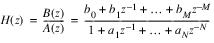
Digital filter approximation problems consist of selecting the coefficients of the rational transfer function H(z):

in order to achieve some desired result when the filter is applied to a signal. All of the filter approximation routines in the PV‑WAVE Signal Processing Toolkit return the filter coefficients in a digital filter data structure.

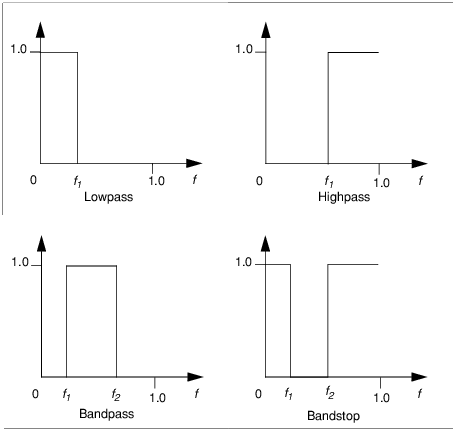
Classical FIR and IIR filter approximation problems concern the approximation of the ideal lowpass, highpass, bandpass, and bandstop filters as illustrated in Figure 1-2: Ideal Filter for FIR and IIR Filter Approximation on page 11.

Figure 1-2: Ideal Filter for FIR and IIR Filter Approximation

A summary of PV‑WAVE Signal Processing Toolkit functions for solving classical filter design problems is listed in the following table. FIR and IIR filter approximations use separate functions in the Signal Processing Toolkit. For detailed information, see Reference (A to F) and Reference (G to P).

Table 1-3: Classical Filter Approximation Functions
Function	Description
BILINTRANS (*)	Bilinear transform
FIRDESIGN (*)	FIR lowpass, highpass, bandpass, bandstop filter design
FIRLS (*)	FIR multiple bandpass FIR filter design
FIRWIN	FIR window functions
FREQTRANS (*)	IIR filter frequency transformation
FREQTRANSDESIGN	IIR filter frequency transformation design for multiple bandpass IIR filter design
IIRDESIGN (*)	IIR Butterworth, Chebyshev I, Chebyshev II, and elliptic filter design
IIRORDER	IIR filter order estimation
* function uses the digital filter data structure

The classical approach to FIR filter design uses window functions. This approach first determines the inverse Fourier transform of the ideal filter frequency response:

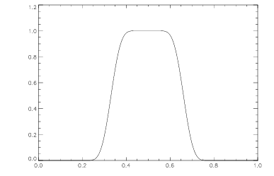
The following example illustrates the design of a windowed bandpass filter. Figure 1-3: Windowed Bandpass Filter Frequency Response on page 13 shows the resulting filter frequency response.

Figure 1-3: Windowed Bandpass Filter Frequency Response

One of the key features of the PV‑WAVE Signal Processing Toolkit is the flexibility of IIR filter design which results from the approach used in applying transformations in IIR filter design. This approach enables you to design all of the filters in the classical approach, and has the added advantage of simplifying the design of multiple bandpass filters.

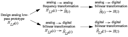
The classical approach to IIR filter design starts with an analog lowpass filter prototype and then applies various frequency transformations to arrive at the desired digital filter. There are two approaches to applying transformations to an analog lowpass filter prototype as illustrated in Figure 1-4: Transformation Application Approaches on page 13. The top path in the figure illustrates the standard approach taken in IIR filter design, and the bottom path illustrates the alternate approach used in the PV‑WAVE Signal Processing Toolkit.

Figure 1-4: Transformation Application Approaches

The approach illustrated in the top path of Transformation Application Approaches is the approach most often employed by signal processors. This standard approach first transforms the analog lowpass filter prototype HLP(s) into an appropriate lowpass, highpass, bandpass, or bandstop filter

The approach used in the Signal Processing Toolkit is shown in the bottom path in Transformation Application Approaches. This alternate approach can design all of the filters available using the standard approach, but has the added advantage of simplifying multiple bandpass filter design. This approach first transforms the analog lowpass filter prototype HLP(s) into a digital lowpass filter prototype:

using the bilinear transform. Then a frequency transformation is applied to obtain an appropriate lowpass, highpass, bandpass, or bandstop digital filter H(z).

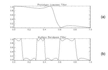
The following example illustrates the ease in designing a multiple bandpass elliptic filter using the PV‑WAVE Signal Processing Toolkit.

In Multiple Bandpass Filter, (a) shows the magnitude frequency response of the original lowpass filter, and (b) shows the response after applying the frequency transformation to obtain the multiple bandpass filter.

Figure 1-5: Multiple Bandpass Filter

The PV‑WAVE Signal Processing Toolkit also includes several advanced filter approximation functions and multirate filter approximation functions.

The advanced filter approximation functions produce filters that are optimal subject to various constraints, such as least-squares error criteria, Chebyshev error criteria, and moment preserving criteria.The least-squares filter approximation functions shown in Advanced Filter Approximation Functions can also be used to obtain filters that interpolate a given set of impulse or frequency response values. For detailed information, see Reference (A to F), Reference (G to P), and Reference (Q to Z).

Table 1-4: Advanced Filter Approximation Functions
Function	Description
FIRLS (*)	Frequency domain least-squares FIR filter design
IIRLS (*)	Frequency and time domain least-squares filter design
REMEZ (*)	Optimal Chebyshev error FIR filter design (Parks-McClellan algorithm)
SGFDESIGN (*)	Optimal Savitsky-Golay FIR filter design
* function uses digital filter data structure

Multirate Filter Approximation Functions shows the list of multirate filter approximation functions that produce filters which are used in standard multirate filtering operations such as decimation and interpolation. For detailed information, see Reference (A to F) and Reference (Q to Z)..

Table 1-5: Multirate Filter Approximation Functions
Function	Description
FILTDOWNDESIGN (*)	Decimation filter design
FILTUPDESIGN (*)	Interpolation filter design
QMFDESIGN (*)	Quadrature mirror filter design
* function uses digital filter data structure