Animation Example
In this example, you’ll experiment with animation using the VDA Tool WzAnimate. You observe the animation in the same manner that you would view a movie—by the rapid display of a series of still graphics.
We chose an example that allows you to observe how a shock wave, radiating through a block of graphite composite, is reflected off the boundaries of the block. You’ll also get some practice adding annotation to a plot.
1. If you are not presently running the Navigator, you will need to start it now. Follow the same procedure to start the Navigator as you followed in the previous two examples.
2. Close any VDA Tools that are currently open.
Importing the Animation Data
Start by importing the multidimensional shock wave data into PV‑WAVE. The data for this exercise has been provided for you as a save file. The data was generated in this format using PV‑WAVE commands.
1. To read the PV‑WAVE save file, enter the following command at the PV‑WAVE prompt:
WAVE> RESTORE, !Data_Dir+'shock_wave.sav'
Now the data is ready to use as a series of PV‑WAVE variables.
2. Click on the WzVariable icon in the Navigator window. The WzVariable Tool appears.
3. Resize the WzVariable Tool by dragging the bottom right corner downward until the window is about six inches long. Resizing allows you to avoid scrolling to select variables.
Note that a series of variables beginning with “DSP” and “STR” appear in the WzVariable Tool list. All of these variables were imported from the same save file.
The variables represent data from 14 time slices taken at 1 millisecond intervals. The variable with the name beginning in DSP contains displacement data. These data values represent the magnitude of the displacement of molecules from their equilibrium position in a plane in the block. The variables with names beginning in STR contain stress data. These data values represent stress on points in the plane.
Each variable contains an array of 55-by-40 displacement or shock values. That is, each of the 55 slices has 40 points at which data was measured.
Viewing Displacement as an Image
To begin, increase the size of the image DSP14 using the REBIN command and then view the image to see what it looks like before you animate it.
1. Enter the following command at the PV‑WAVE prompt:
WAVE> DSP_MAG = REBIN(DSP14, 55*10, 40*10)
This increases the size by a factor of ten. Remember that with REBIN, any array you create must be a multiple or factor of the original array.
2. In the WzVariable Tool, select Options=>Redisplay List. The newly created variable now appears in the list.
3. Click on the DSP_MAG variable in the WzVariable Tool. Now that variable is selected and ready to be displayed as an image.
4. Click the WzImage icon in the Navigator window. The image is displayed in the WzImage Tool.
5. Click the WzColorEdit icon in the Navigator window.
6. Select
Colortable=>System, and then select
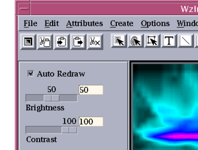
Blue-Red from the colortable list. You’ll notice that the color of the image has changed to blue and red as shown in
Table C-19: Displacement Data on page 260.
7. Click on Dismiss in the System Colortable list.
8. Close the WzColorEdit Tool
9. Close the WzImage Tool.
Shading and Rotating a Surface View
Now create a surface view using two variables. Use DSP14 for the surface, and shade it using STR14. By shading the surface, you create a view that contains more information than can be obtained from either variable alone.
1. In the WzVariable Tool list, select DSP14.
2. Click the WzSurface icon in the Navigator window.
3. Select Attributes=>Surface Attributes from the WzSurface menu bar. The Surface Attributes dialog box appears. Now select your view attributes by interacting with some option menus.
4. Select None for the Surface attribute (in the Surface option menu in the dialog box).
5. Now select From Variable from the Shading option menu.
6. Type STR14 in the Shade Variable text input field.
The default view displays a surface at a 30 degree angle of rotation about the Z axis, which is displayed as the vertical axis. However, your individual surface plot might be better viewed from a different angle. The WzSurface Tool lets you rotate to any view angle.
Practice changing the rotation by changing the angle to 120 degrees.
1. Select the value 30 next to the Z Rotation slider and change the value to 120. Press <Return> to confirm the rotation change.
2. When you finish viewing the surface, close the WzSurface Tool.
Building an Animation Sequence
Next, you will create an animation sequence with the WzAnimate Tool. You individually create the frames that will be animated and store them in a variable. After the sequence is complete, you can animate the frames forward or backward. WzAnimate displays the views in rapid sequence, allowing you to get a dynamic, interactive view of your data.
For this example, you’re animating surface views of the data. The first step is to create an animation array.
Defining an Animation Array
You will create the array at the same time that you store the first frame. Your animation sequence will consist of six “snapshots” of the shock wave.
1. Select STR01 in the WzVariable list.
3. In the WzSurface Tool, select File=>Export As Pixmap. The Export Pixmap dialog box appears. Note that the name ANIMATE_0 appears in the Pixmap Variable Name text field, and the Add to Pixmap Variable button is selected.
4. Click Apply. At this point, the plot in the WzSurface display area is saved as a pixmap in the variable called ANIMATE_0.
5. Select STR02 through STR06 in the WzVariable list. To select multiple elements of a list, click MB1 on the first element, and click Shift-MB1 on each subsequent element.
6. Select File=>Export Variables in the WzVariable Tool.
7. In the Export Variables dialog box, select STR02 in the upper list box and make sure that WzSurface_0 is selected in the lower list box.
8. Click Apply in the Export Variables dialog box. This exports the variable STR02 to the WzSurface Tool, which displays the variable in its view area.
9. Click the Apply button in the Export Pixmap dialog box. Now, you have stored a second pixmap in the variable ANIMATE_0.
10. Repeat steps 7, 8, and 9 four more times, each time selecting the next variable, until STR03, STR04, STR05, and STR06 are stored in ANIMATE_0.
11. When you have saved all variables, close the Export Pixmap dialog box by clicking the Cancel button.
12. Close the Export Variables dialog box by clicking the Cancel button.
13. Select Options=>Redisplay List in the WzVariable Tool. The variable ANIMATE_0 appears in the list.
14. Double-click on the variable name ANIMATE_0 in the WzVariable list. The Variable Information dialog box confirms that this is a 3D variable (640-by-512-by-6). The first two dimensions hold the image data, and the third dimension represents the number of individual pixmaps in the animation sequence. For example, if the dimensions of a variable were 512-by-512-by-30, the variable, when viewed in the WzAnimate Tool, would produce a loop or cycle consisting of 30 frames.
15. Click OK to dismiss the Variable Information dialog box.
16. Close the WzSurface Tool.
You have now stored a six-frame animation sequence. You are ready to view the animation sequence.
Viewing Animation
Now view the animation to see how the shock wave develops.
Since you did not define an animation array name, the array was given the default name, ANIMATE_0.
1. In the WzVariable Tool, select ANIMATE_0 from the list. Ensure that all other variables are deselected.
2. Click the
WzAnimate icon in the Navigator window. The WzAnimate Tool appears as shown in
Table C-22: WzAnimate Tool on page 265. Now you’re ready to play the animation in a variety of ways:
3. Select the Continuous button in the controls area.
4. Select the Forward button to run the animation frames forward. You may want to try some of the other animation controls, such as the Reverse button and the Stop button.
5. When you are finished viewing the animation, select the Stop button and then close the WzAnimate Tool.
Changing the Appearance of a Plot
After a plot is created, you can change its appearance and annotate it. For example, you may want to do this before showing the plot to someone else, before printing it for your files, or to prepare an illustration for a publication.
For this example, you can use a surface view of STR14. You’ll change the colors of parts of the plot, select a font to use for a title you’re giving the plot, and place the title on the plot.
1. Select STR14 from the WzVariable list. Make sure that all other variables are deselected.
2. Click the WzSurface icon in the Navigator window.
3. Select Attributes=>Surface Attributes. The Surface Attributes dialog box appears. This dialog box offers a variety of options to enhance the appearance of a plot. We’ll suggest a particular set of attributes, but you may want to experiment using your own attributes.
4. Click the Upper Color button and select the color white from the color bar, then click OK. This choice will make the top of the surface white (color 1).
5. Click the Lower Color button and select the color red from the color bar, then click OK. This choice will make the base (underside) of the surface red (color 3).
6. Select the Skirt checkbox to highlight the edge of the surface with a skirt.
7. Select the OK button of the Surface Attributes dialog box to apply the attributes and exit the dialog box.
8. Select Attributes=>View Attributes.
9. Click the Background Color button and select the color blue (color 5) from the color bar, then click OK.
10. Click OK in the View Attributes dialog box.
Now add a title to your plot.
1. Select Attributes=>Defaults=>Text Object. The Default Text Attributes dialog box appears.
2. Click the Color button and select the color cyan (color 6) from the color bar, then click Dismiss.
3. Select Complex Roman from the Font option menu.
4. Enter 2 in the Size field and 2 in the Thickness field.
5. Click the OK button.
6. Select the Create Text Object icon on the WzSurface Tool button bar, or select Create=>Text Object.
7. Position the pointer near the upper-left corner of the plot and click MB1. Then type Shockwave Displacement Magnitude and press <Return>.
The surface plot of
STR14 now includes a title at the top of the plot as shown in
Changed Plot.
Saving and Using a Template
Now that you have a surface plot set up with annotation, colors, and other attributes, you can save these setups as a template. Then, you can open other surface plots with the template, and those plots will contain the same color, text, and other setups.
This feature can be useful if you want to achieve a consistent look or style in your graphics output. For example, you could create a template with a custom legend in one corner and a company logo in another.
1. Select File=>Save Template As from the Navigator menu bar. The Save Template dialog box appears.
2. In the Enter File Name field, enter the name of a file for the template. Give the filename a .tpl extension, for example STR14.tpl.
3. Click OK. Now that the template is saved, you can use it with other surface plots.
4. Close the WzSurface Tool.
5. Select Defaults=>WzSurface from the Navigator menu bar. The Default VDA Tool Attributes dialog box appears.
6. In the Template File Name field, enter STR14.tpl (or whatever you named the template file). Or, you can use the Browse button to locate and select the file.
7. Click OK.
8. In the WzVariable Tool, select STR13.
9. Click the WzSurface icon in the Navigator window.
A new surface appears with all the same annotations and other setups that were saved in the template.
Saving a Plot
You can save a specific plot, along with all of its annotation and other attributes, for future use in another application, such as a desktop publishing system.
1. To save the plot, select File=>Print Setup. The Printer Setup dialog box appears. On Windows, use File=>Print.
2. Select Postscript from the Printer Type option menu.
3. Select the Print to file button and type shock_wave_plot in the Print to file text field, then select the OK button. The plot is saved as a PostScript file.
4. Close the WzSurface Tool.
PostScript files can be saved in three different formats; you make your choice with an option menu in the Postscript Options dialog box. This dialog box is displayed when you select the Options button in the Printer Setup dialog box.
Encapsulated or encapsuled interchange (EPSI) PostScript files can be used with other applications. For example, you may want to import the file directly into a desktop publishing system to prepare a publication with embedded graphics. If you export the file with the EPSI option enabled, some publishing systems will be able to display the plot on the screen, as well as having it appear in the hardcopy output.
Experimenting on Your Own
By now, you have a good idea of how to use the Navigator and VDA Tools.
VDA Tools provide a rich environment for doing visual data analysis. This tutorial covered only a portion of the VDA Tool capabilities. We encourage you to try out the following features. You can read more about them in the online help system:
 Code generation
—Save the PV‑WAVE code used to create a plot in a file. You can then use this code in other applications.
Copy and paste between VDA Tools—You can copy graphical elements such as text, lines, and rectangles from one VDA Tool and paste them in another VDA Tool.
Histogram plots—Try out the WzHistogram Tool. Use it to analyze quantitative trends in large datasets.
Contour plots—The WzContour Tool displays 2D variables containing contour data.
Data export—The WzExport Tool can be used to export data from a variable to a file.
Exiting PV-WAVE
To exit PV‑WAVE, type EXIT at the WAVE> prompt.
Version 2017.1
Copyright © 2019, Rogue Wave Software, Inc. All Rights Reserved.