Lesson 2: Read and Plot Data
Perhaps one of the most common, and certainly one of the most useful, ways to display data is with the simple linear plot.
This example demonstrates how to plot the data, smooth the noisy data, then replot the data as a velocity field. The following activities are performed in this example:
Process and Plot the Signal Data
To process and plot the signal data, do the following:
2. Load a colortable that specifies the first 32 distinct colors in the lower end of the colortable:
TEK_COLOR
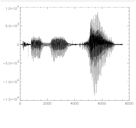
3. To view a quick plot of this data set, enter:
PLOT, original
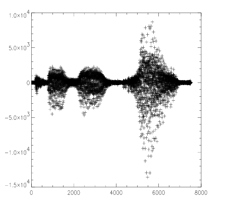
4. Now add some uniformly-distributed random noise to this data set; store it in a new variable by entering:
noisy = original + (RANDOMU(seed, sig_len)*1000)-500
The RANDOMU function creates an array of uniformly distributed random values. The original data set plus the noise is stored in a new variable called noisy.
5. Plot noisy and specify a color for drawing it:
PLOT, noisy, Color=WoColorConvert(2), Psym=1
6. Display the original data set and the noisy version simultaneously by entering the following:

Plot the
original data again, this time with titles.
PLOT, original, XTitle='Time', YTitle='Amplitude'
Overplot the
noisy data as points, using crosses to mark the points.
OPLOT, noisy, Color=WoColorConvert(4), PSym=1
The XTitle and YTitle keywords are used to create the x and y axis titles. The OPLOT command is used to plot the noisy data set over the existing plot of original without erasing.
Smooth the Data
A simple way to smooth the noisy data set is to use PV-WAVE’s SMOOTH routine, which returns a copy of an array smoothed with a boxcar average of a specified width.
To smooth noisy data, do the following:
1. Create a new variable to hold the smoothed data set and display it by entering the following commands:
smoothed = SMOOTH(noisy, 5)
2. Plot the smoothed data in a different color:
PLOT, smoothed, PSym=1, Color=WoColorConvert(3)
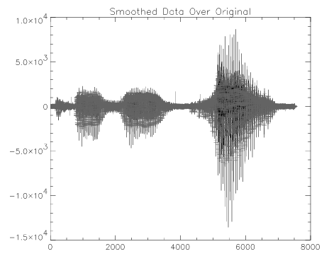
3. Compare the smoothed data to the original by overplotting it on the original data and add a title:
PLOT, original, Title="Smoothed Data Over Original"
OPLOT, smoothed, PSym=1, Color=WoColorConvert(3)
The Title keyword draws the title text centered above the plot, and the smoothed line appears less jagged than the original.
Notice that while SMOOTH did a fairly good job of removing noise spikes, the resulting amplitudes “taper off” as the frequency increases as shown in
Smoothed Data Overplotted on Original Data.
Plot the Data as a Velocity Field
An example of a more complicated plotting routine written in PV-WAVE is the VEL routine from the PV-WAVE Standard Library. The Standard Library contains many useful functions and procedures written with the PV-WAVE language. The VEL routine plots velocity vectors given arrays of x and y velocity values.
To plot the signal data as a velocity field, do the following:
1. Create a dummy set of x and y velocities to visualize by entering:
VX = original#FINDGEN(20)
VY = noisy#FINDGEN(20)
The PV-WAVE matrix multiplication operator (#) is used to make the needed dummy arrays.
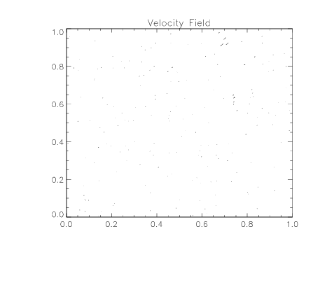
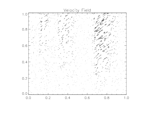
2. Now use the VEL command to plot the velocity vectors by entering:
VEL, VX, VY
The information is plotted, with the length of each arrow following the velocity field and being proportional to the field strength. The results are shown in
Velocity Vectors Plot.
For most plots, the default appearance is adequate. Nevertheless, you can make the plot more informative by adding a few keywords to the command line.
3. Specify the length of the lines to be five times as long as the default value (0.1) and specify the number of points to be plotted as six times the default value (200):
VEL, VX, VY, Length=.5, NVecs=1200
Version 2017.1
Copyright © 2019, Rogue Wave Software, Inc. All Rights Reserved.