Drawing Contour Plots with CONTOUR
The following sections describe how to use the CONTOUR procedure; however, most of the information applies to CONTOUR2 as well. The primary differences between CONTOUR and CONTOUR2 are listed in the previous section. For detailed information on these procedures, see the PV-WAVE Reference.
The CONTOUR procedures draw contour plots from data stored in a rectangular array. In their simplest form, these procedures make a contour plot given a two-dimensional array of z values. In more complicated forms, CONTOUR accept, in addition to z values, arrays containing the x and y locations of each column, row, or point, plus many keyword parameters. In more sophisticated applications, the output of CONTOUR may be projected from three dimensions to two dimensions, superimposed over an image, or combined with the output of SURFACE.
Basic Usage
The simplest call to CONTOUR is:
CONTOUR, z
This call labels the x– and y–axes with the subscript along each dimension. For example, when contouring a 10-by-20 array, the x–axis ranges from 0 to 9, and the y–axis from 0 to 19.
You can explicitly specify the x and y locations of each cell with the call:
CONTOUR, z, x, y
The x and y arrays may be either vectors or two-dimensional arrays of the same size as z. If they are vectors, the element Zi,j has a coordinate location of (Xi, Yj). Otherwise, if the x and y arrays are two-dimensional, the element Zi,j has the location (Xi,j, Yi,j). Thus, vectors should be used if the x location of Zi,j does not depend upon j and the y location of Zi,j does not depend upon i.
Dimensions must be compatible. In the one-dimensional case, x must have a dimension equal to the number of columns in z, and y must have a dimension equal to the number of rows in z. In the two-dimensional case, all three arrays must have the same dimensions.
PV‑WAVE uses linear interpolation to determine the x and y locations of the contour lines that pass between grid elements. The cells must be regular, in that the x and y arrays must be monotonic over rows and columns, respectively. The lines describing the quadrilateral enclosing each cell and whose vertices are (Xi,j, Yi,j), (Xi+i,j, Yi+1,j), (Xi+1,j+i, Yi+i,j+i), and (Xi,j+1, Yi,j+1) must intersect only at the four corners.
Alternative Contouring Algorithms in CONTOUR
In order to provide a wide range of options, CONTOUR uses either the cell drawing or the follow method of drawing contours.
Cell Method
The cell drawing method is used by default. It examines each array cell and draws all contours emanating from that cell before proceeding to the next cell. This method is efficient in terms of computer resources but does not allow such options as contour labeling or smoothing.
Follow Method
The follow method searches for each contour line and then follows the line until it reaches a boundary or closes. This method gives better looking results with dashed linestyles, and allows contour labeling and bicubic spline interpolation, but requires more computer time. It can be used in with the CONTOURFILL procedure to shade closed contour regions with specified colors, as explained in
"Filling Contours with Color". The follow method is used if any of the following keywords is specified:
C_Annotation,
C_Charsize,
C_Labels,
Follow,
Path_Filename, or
Spline. In addition, the use of any of these keywords causes the contours to be labeled.
note | Because of their differing algorithms, these two methods will often draw slightly different correct contour maps for the same data. This is a direct result of the fact that there is often more than one valid way to draw contours, and should not be a cause for concern. |
Controlling Contour Features with Keywords
In addition to most of the keyword parameters accepted by PLOT, the following keywords apply to CONTOUR.
C_Annotation | C_Labels | Follow | NLevels |
C_Charsize | C_Linestyle | Levels | Path_Filename |
C_Colors | C_Thick | Max_Value | Spline |
For a detailed description of these keywords, see Chapter 21: Graphics and Plotting Keywords from the PV‑WAVE Reference.
Contouring Example
Digital elevation data of the Maroon Bells area, near Aspen, Colorado, are used to illustrate the CONTOUR procedure. This data provides terrain elevation data over a 7.5 minute square (approximately 11-by-13.7 kilometers at the latitude of Maroon Bells), with 30 meter sampling measured in Universal Transverse Mercator (UTM) coordinates.
The data are read into a 350-by-460 array A. The rectangular array is not completely filled with data, because the 7.5 minute square is not perfectly oriented to the UTM grid system. Missing data are represented as zeroes. Elevation measurements range from 2658 to 4241 meters, or from 8720 to 13,914 feet.
Figure 5-1: Maroon Bells Contour Plot on page 86 is the result of applying the CONTOUR procedure to the data, using the default settings:
CONTOUR, A
A number of problems are apparent:

PV‑WAVE selected six contour levels, by default, of (4241 – 0) / 7 meter intervals, or approximately 605 meters. The levels are 605, 1250, ..., 3635, meters, even though the range of valid data is from 2658 to 4241 meters. This is because the missing data values of 0 were considered when selecting the intervals. It is more appropriate to select levels only within the range of valid data.
For most display systems, and for contour intervals of approximately 200 meters, the data are oversampled in the XY direction. This oversampling has two adverse effects: the contours appear jagged, and a large number of short vectors are produced. This can cause performance problems when you attempt to plot the data on a graphics device, especially if the graphic output is directed to a serial terminal or PostScript printer.
The axes are labeled by point number, but should be in UTM coordinates.
It is difficult to visualize the terrain and to discern maxima from minima because each contour is drawn with the same type of line.
Each of the above problems is readily solved using the following simple techniques:
Specify the contour levels directly using the
Levels keyword parameter. Selecting contour intervals of 250 meters, at elevation levels of [2750, 3000, 3250, 3500, 3750, 4000], results in six levels.
Change the missing data value to a value well above the maximum valid data value. Then use the
Max_Value keyword parameter to exclude missing points. In this example, we set missing data values to one million with the statement:
A(WHERE(A EQ 0)) = 1.0E6
Use the REBIN function to decrease the sampling in
x and
y by a factor of 5:
B = REBIN(A, 350/5, 460/5)
This smooths the contours, because the call to REBIN averages 52 = 25 bins when resampling. The number of vectors transmitted to the display are also decreased by a factor of approximately 25. The variable B is now a 70-by-92 array.
Care was taken, in the second step, to ensure that the missing data is not confused with valid data after REBIN is applied. As, in this example, REBIN averages bins of 52 = 25 elements, the missing data value must be set to a value of at least 25 times the maximum valid data value. After application of REBIN any cell with a missing original data point will have a value of at least 106/25 = 40000, well over the largest valid data value of approximately 4500.
Vectors
x and
y are constructed containing the UTM coordinates for each row and column. From the USGS data tape, the UTM coordinate of the lower-left corner of the array is (326850, 4318500) meters. As the data spacing is 30 meters in both directions, the
x and
y vectors, in kilometers, are easily formed using the FINDGEN function, as shown in the following example.
Contour levels at each multiple of 500 meters (every other level), are drawn with a solid line style, while levels in between are drawn with a dotted line style. In addition, the 4000 meter contour is drawn with a triple thick line, emphasizing the top contour.
The result of these improvements is
Figure 5-2: Improved Contour Plot on page 88. It was produced with the following statements:
; Set missing data points to a large value.
a(WHERE(a eq 0)) = 1e6
; Rebin down to a 70-by-92 matrix.
b = REBIN(a, 350/5, 460/5)
; Make the x and y vectors, giving the position of each
; column and row.
x = 326.850 + .030 * FINDGEN(70)
y = 4318.500 + .030 * FINDGEN(92)
; Make plot, specifying contour levels, missing data value,
; line styles, etc. Set style keywords to 1, for exact axes.
CONTOUR, b, x, y, Levels = 2750+FINDGEN(6) * 250., XStyle = 1, $
YStyle = 1, Max_Value = 5000, $
C_Linestyle = [1, 0, 1, 0, 1, 0], $
C_Thick = [1, 1, 1, 1, 1, 3], Title = 'Maroon Bells Region', $
Subtitle = '250 meter contours', $
XTitle = 'UTM Coordinates (KM)'
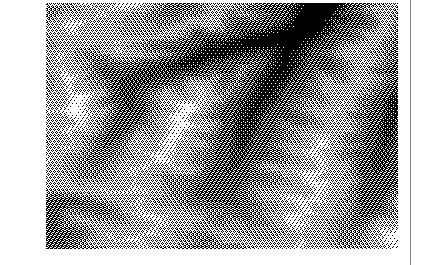
Overlaying Images and Contour Plots
Maroon Bells illustrates the data displayed as a gray-scale image. Higher elevations are white. This image demonstrates that contour plots do not always provide the best qualitative visualization of many two-dimensional data sets.
Superimposing an image and its contour plot combines the best of both worlds; the image allows easy visualization, and the contour lines provide a semi-quantitative display.
note | Beginners may want to skip the programs presented in the rest of this section. A combined contour and image display, such as that discussed in this section, can be created using the IMAGE_CONT procedure. The following material is intended to illustrate the many ways in which images and graphics may be combined using PV‑WAVE. |
The technique used to overlay plots and images depends on whether or not the device is able to represent pixels of variable size, as does PostScript, or if it has pixels of a fixed size. If the device does not have scalable pixels the image must be resized to fit within the plotting area (if it is not already of a size suitable for viewing). This leads to three separate cases which are illustrated in the following examples.
Overlaying on Devices with Scalable Pixels
Certain devices, notably PostScript, can display pixels of any given size. With these devices, it is easy to set the size and position of an image so that it exactly overlays the plot window. For example, the following statements produce
Figure 5-4: Image and Contour Overlay on page 90:
; Scale the range of valid elevations into intensities.
c = BYTSCL(a, MIN = 2658, MAX=4241)
; Display image with its lower-left corner at the origin of the
; plot window, and with its size scaled to fit the plot window.
TV, c, !X.Window(0), !Y.Window(0), XSize = !X.Window(1) - $
!X.Window(0), YSize = !Y.Window(1) - !Y.Window(0), /Norm
; Write the contours over the image, being sure to use the exact
; axis styles so that the contours fill the plot window. Inhibit
; erasing.
CONTOUR, b, x, y, Levels = 2750+FINDGEN(6) *250., $
MAX_VALUE = 5000, XStyle = 1, YStyle =1, /Noerase, $
Title = 'Maroon Bells Region', $
Subtitle = '250 meter contours', $
XTitle = 'UTM Coordinates (KM)'
Be sure that the position of the plot window contained in the field Window in !X, !Y, and !Z, is set, using CONTOUR or PLOT, before executing the above statements.
Also, note that in
Image and Contour Overlay that the aspect ratio of the image was changed to fit that of the plot window. If it is desired to retain the original image aspect ratio, the plot window must be resized to an identical aspect ratio using the
Position keyword parameter.
Overlaying on Devices with Fixed Pixels
There are two methods for overlaying images on devices with fixed pixels.
Method 1
If the pixel size can't be changed, for example on a Sun workstation monitor, an image of the same size as the plotting window must be created using the POLY_2D function. The REBIN function can also be used to resample the original image, if the plot window dimensions are an integer multiple or factor of the original image dimensions. REBIN is always faster than POLY_2D.
The following commands create an image of the same size as the window, display it, and then overlay the contour plot. These commands perform the same basic function as the IMAGE_CONT procedure, which is described in the PV‑WAVE Reference.
; Get size of plot window in device pixels.
px = !X.Window * !D.X_Vsize
py = !Y.Window * !D.Y_Vsize
; Desired size of image in pixels.
sx = px(1)-px(0)+1
sy = py(1)-py(0)+1
; Get size of original image. sz(1) = number of columns,
; sz(2) = number of rows.
sz = SIZE(a)
; Erase the display.
ERASE
; Create a sx-by-sy image stretched from the original. Display it
; with same lower-left corner coordinate as the window. Note that
; we BYTSCL before changing the size, as it is more efficient to
; apply POLY_2D to byte images. Also, it is likely that the
; original image is smaller than the stretched image.
TV, POLY_2D(BYTSCL(a), [[0,0], [sz(1)/sx,0]], $
[[0,sz(2)/sy],[0,0]], 0, sx, sy), px(0), py(0)
; Draw the contour without first erasing the screen.
CONTOUR, a, /Noerase, XStyle = 1,YStyle = 1
Method 2
If the image is already close to the proper display size, it is simpler and more efficient to change the plot window size to that of the image. The following commands display the image at the window origin, and then set the plot window to the image size, leaving its origin unchanged:
; Get the size of the plot window in device pixels.
px = !X.Window * !D.X_Vsize
py = !Y.Window * !D.Y_Vsize
; The size of the original image.
sz = SIZE(a)
ERASE
; Scale and display image at lower left corner of plot window.
TVSCL, a, px(0), py(0)
; Make contour, explicitly set plot window, in device coordinates
; to the size of the image. Make the axes exact. Don't erase.
CONTOUR, a, /Noerase, XStyle = 1, YStyle = 1, $
Position = [px(0), py(0), px(0)+sz(1)-1, $
py(0)+sz(2)-1], /Device
Of course, by using other keyword parameters with the CONTOUR procedure, you can further customize the results.
Labeling Contours
In the following discussion, a variable named DATA is contoured. This variable contains uniformly distributed random numbers obtained using the following statement:
DATA = RANDOMU(SEED, 6, 6)
note | The default SEED value is used to create the DATA variable. Because of this, if you try to run these examples, your output will probably differ somewhat from the illustrations shown. |
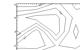
To label contours using the defaults for label size and contours to label, it is sufficient to simply select the
Follow keyword. In this case, CONTOUR labels every other contour using the default label size (3/4 of the plot axis label size). Each contour is labeled with its value.
Labeled Contour Plot was produced using the statement:
CONTOUR, /Follow, DATA
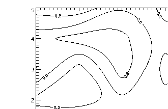
The C_Charsize keyword is used to specify the size of the characters used for labeling, in the same manner that Size is used to control plot axis label size. The C_Labels keyword can be used to select the contours to be labeled. For example, suppose that we want to contour the variable DATA at 0.2, 0.5, and 0.8, and we want all three levels labeled. In addition, we wish to make each label larger, and use PostScript fonts. This can be accomplished with the statement:
; Note that Font = 0 is used to specify the use of hardware fonts.
CONTOUR, Level = [0.2, 0.5, 0.8], C_Labels = [1, 1, 1], $
C_Charsize = 1.25, DATA, Font = 0
For more information on hardware fonts, see
"Software vs. Hardware Fonts: How to Choose". The result of this statement is shown in
Modified Labels.
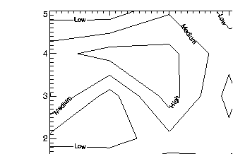
Finally, it is possible to specify the text to be used for the contour labels using the C_Annotation keyword.
CONTOUR, Level = [0.2, 0.5, 0.8], C_Labels = [1, 1, 1], $
C_Annotation = ['Low', 'Medium', 'High'], DATA, Font = 0
The result is shown in
Specified Labels.
Smoothing Contours
The CONTOUR2 algorithm produces smoothed contour lines by default.
When the Spline keyword is specified, CONTOUR smooths the contours using cubic splines. This is especially effective when used with sparse data sets—the effectiveness of smoothing diminishes if enough data points are present and the cost of the spline calculations increases. Use of spline interpolation is not recommended when the array dimensions are more than approximately 15.
The effect of smoothing the variable DATA using the statement:
CONTOUR, Level = [0.2, 0.5, 0.8], C_Labels = [1, 1, 1], $
/Spline, DATA
can be seen in
Smoothed Contour Plot. Compare it with the non-smoothed versions in
Modified Labels and
Specified Labels.
Filling Contours with Color
The following procedure applies primarily to CONTOUR. The CONTOUR2 procedure simplifies contour filling with a convenient Fill keyword. See the PV-WAVE Reference for information filling contours with CONTOUR2.
It is possible to fill closed contours with color by using the keyword Path_Filename in conjunction with the procedure COUNTOURFS. Path_Filename specifies the name of a file to contain the contour positions. If Path_Filename is present, CONTOUR does not draw the contours, but rather, opens the specified file and writes the positions, in normalized coordinates, into it. COUNTOURFS uses this file to fill the closed contours with different colors. COUNTOURFS has the form:
CONTOURFS, filename[, Color_Index = cin]
where filename is the name of the file written by CONTOUR and cin is the color index array. Element 0 of cin contains the background color, and each of the following elements contains the color that the corresponding contour level should be filled with. If the Color_Index keyword is not specified, COUNTOURFS supplies a default set of colors.
The problem with directly producing a plot in this manner is that most of the contours are not closed, as they run beyond the borders of the plot. Since COUNTOURFS can only fill closed contours, many of the contours will not be filled. This can be avoided by creating an array with two more columns and two more rows than our data array. The data array is placed into the center of this new array, and the outer rows and columns are set to a value that is not specified in the Levels keyword. This will ensure that there are no open contours. To demonstrate with our DATA variable:
; DATA2 has two more rows and two more columns than DATA, and
; is filled with –1.0, which is not a value that will be specified
; as a contour level.
data2 = REPLICATE(-1.0, 8, 8)
; DATA is copied into center of DATA2. The edges remain at –1.0.
data2(1,1) = data
Using DATA2, the following statements will produce a contour plot of DATA with the contours filled:
; Levels to contour.
clev = [0.2, 0.5, 0.8]
; Colors to fill with.
cin = [192, 208, 224, 240]
; Contours to Label (all three specified in clev).
clab=[1, 1, 1]
; Create file named cpaths.dat containing contour paths. The
; range keywords avoid plotting top and right border. The style
; keywords prevent PV‑WAVE from rounding plot range to a
; different value from that specified. CONTOURFS fills closed
; contours and draws the contours over the filled regions.
CONTOURFS, /Spline, Levels = clev, C_Label = clab, $
Path_Filename = 'cpaths.dat', data2, XRange = [0, 7], $
XStyle = 1, YRange = [0, 7], YStyle = 1, Col_Index = cin
The result is shown in
Filled Contour Plot.
Version 2017.1
Copyright © 2019, Rogue Wave Software, Inc. All Rights Reserved.