Creating Basic 3D Plots
This section describes the basic 3D plots you can create with PV-WAVE. The 3D plotting procedures include:

CONTOURFS—Draws contour plots.
SURFACE—Draws 3D surface plots.
SHADE_SURF—Draws shaded 3D surface plots.
CONTOURFS and SURFACE use line graphics to depict the value of a two-dimensional array. As the name implies, CONTOURFS draws contour plots. SURFACE depicts the surface created by interpreting each array element as an elevation. SURFACE projects this three-dimensional surface, after an arbitrary rotation about the x– and z–axis, into two dimensions. It then connects each point with its neighbors using hidden line removal. SHADE_SURF provides a shaded surface.
Almost all of the information concerning coordinate systems, keyword parameters, and system variables that are discussed in
Programming with PV-WAVE also apply to CONTOURFS and SURFACE. The keywords and system variables discussed in this chapter are described in detail in the PV‑WAVE
Reference.
This section demonstrates how to create the following types of 2D Plots:
Contour Plots
The CONTOURFS procedures draw contour plots from data stored in a rectangular array. In their simplest form, these procedures make a contour plot given a two-dimensional array of z values. In more complicated forms, CONTOURFS accepts, in addition to z values, arrays containing the x and y locations of each column, row, or point, plus many keyword parameters. In more sophisticated applications, the output of CONTOURFS may be projected from three dimensions to two dimensions, superimposed over an image, or combined with the output of SURFACE.
CONTOURFS draws contours using one of two different methods:
The first method, used by default, examines each array cell and draws all contours emanating from that cell before proceeding to the next cell. This method is efficient in terms of computer resources, but does not allow contour labeling.
The second method searches for each contour line and then follows the line until it reaches a boundary or closes. This method gives better-looking results with dashed line styles, and allows contour labeling, but requires more computer time. It is used if any of the following keywords is specified:
C_Annotation,
C_Charsize,
C_Charthick,
C_Labels,
Follow,
Spline, or
Path_Filename.
Although these two methods both draw correct contour maps, differences in their algorithms can cause small differences in the resulting graph.
Basic Usage
This example creates a filled contour plot of a 10 by 10 array of random numbers.
b = RANDOMU(seed, 10,10)
; To create a filled contour plot, call CONTOURFS using
; the Path_Filename keyword
CONTOURFS, b, Path_file='path.dat', /XStyle, /YStyle, $
NLevels=5, Col_Index=[2, 3, 4, 5, 6, 7]
Surface Plots
The SURFACE procedure draws “wire mesh” representations of functions of X and Y, just as CONTOURFS draws their contours. SURFACE parameters are similar to CONTOURFS parameters. SURFACE accepts a two-dimensional array of Z (elevation) values, and optionally x and y parameters indicating the location of each Z element.
SURFACE projects the three-dimensional array of points into two dimensions after rotating about the Z and then the X axes. Each point is connected to its neighbors by lines. Hidden lines are suppressed. The rotation about the X and Z axes can be specified with keywords, or a complete three-dimensional transformation matrix can be stored in the field !P.T, for use by SURFACE. Details concerning the mechanics of 3D projection and rotation are covered in the PV‑WAVE User’s Guide.
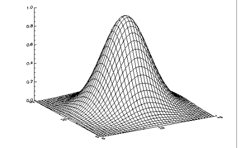
The following code illustrates the most basic call to SURFACE. It produces a two-dimensional Gaussian function and then calls SURFACE to produce
Gaussian Surface Plot.
; Create 40-by-40 array, shift origin to center of array.
z = SHIFT(DIST(40), 20, 20)
; Form Gaussian with 1/e width of 10, and call SURFACE to display.
SURFACE, EXP(-(z/10)^2)
Shaded Surface Plots
The SHADE_SURF procedure creates a shaded representation of a surface made from regularly gridded elevation data. The shading information may be supplied as a parameter or computed using a light source model. Displays are easily constructed depicting the surface elevation of a variable shaded as a function of itself or another variable. This procedure is similar to SURFACE, but it renders the visible surface as a shaded image rather than a mesh.
Parameters are identical to those of the SURFACE procedure, described in
"Surface Plots", with the addition of two optional keywords:
Shades—Specifies an array of the same dimensions as the Z parameter, which contains the shading color indices. This array should be scaled into the range of color indices, normally 0 to 255.
Image—Specifies the name of a variable into which the image created by SHADE_SURF is placed. Normally, the image is displayed on the currently selected graphics device and then discarded.
The left side of
Shaded 2D Gaussian Plots illustrates the application of SHADE_SURF, with light source shading, to the two-dimensional Gaussian,
z, used to produce
Figure 6-1: Gaussian Surface Plot on page 84. This figure was produced by the statement:
SHADE_SURF, z
The right half of
Shaded 2D Gaussian Plots shows the use of an array of shades, which in this case is simply the surface elevation scaled into the range of bytes. The output of SURFACE is superimposed over the shaded image with the statements:
; Show Gaussian with shades created by scaling elevation into the
; range of bytes.
SHADE_SURF, z, SHADE=BYTSCL(z)
; Draw the mesh surface over the shaded figure. Suppress the axes.
SURFACE, z, XSTYLE=4, YSTYLE=4, ZSTYLE=4, /Noerase
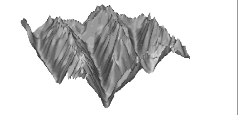
Shaded Surface of Maroon Bells shows the Maroon Bells data as a light source shaded surface. It was produced by the statement:
SHADE_SURF, b, x, y, AZ=210, AX=45, XSTYLE=4, YSTYLE=4, ZSTYLE=4
where b is the 2D array containing the Maroon Bells data. The AX and AZ keywords specify the orientation. The axes are suppressed by the axis style keyword parameters, as in this orientation the axes are behind the surface.
Version 2017.1
Copyright © 2019, Rogue Wave Software, Inc. All Rights Reserved.