Lesson 1: Surface Plotting
This lesson demonstrates how to plot the surface of Pikes Peak, a mountain in Colorado. In this lesson, you’ll do the following:
Access the Data and Create Arrays
First, you need a 2D data set to visualize. This example is a freely formatted file of the Pikes Peak, Colorado, region. The data set contains information about latitude, longitude, elevation, and snow depth, with 2400 single values per variable. This file is located in <RW_DIR>\wave\data, where <RW_DIR> is your installation directory.
To access the data, do the following:
1. Read the data file, using status as the value returned by DC_READ_FREE. Enter:
status = DC_READ_FREE(!Data_Dir + 'wd_pike_elev.dat', $
lat, lon, elev, depth, /Column)
2. Use the INFO command to verify that the new variables lat, lon, elev, and depth were created. This command also tells you about the size and data type of the arrays:
INFO
3. Create four 2D arrays to contain the data. Use the REFORM function to reformat the 1D arrays without changing the values numerically:
lat = REFORM(lat, 60, 40)
lon = REFORM(lon, 60, 40)
elev = REFORM(elev, 60, 40)
depth = REFORM(depth, 60, 40)
4. Enter the INFO command again to see how the arrays have been changed:
INFO
Create a Surface Plot
To create a surface plot, do the following:
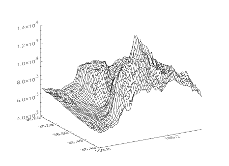
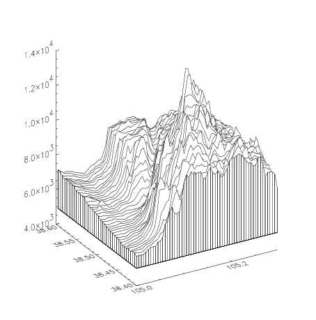
1. To view the array elev as a 3D, wire-frame surface, enter the command:
SURFACE, elev
A wire-frame representation of the array is displayed.
The SURFACE command can be used to view your data from any angle.
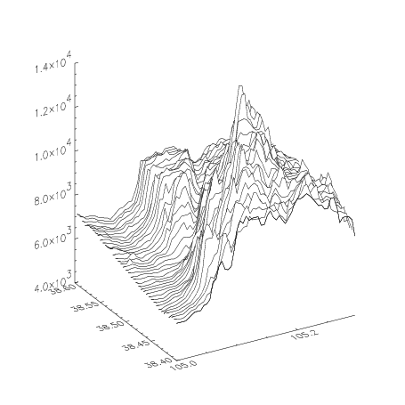
2. Add the latitude and longitude information:
SURFACE, elev, lon, lat
The x- and y-axes of the new plot contain the latitude and longitude information.
SURFACE, elev, lon, lat, XStyle=1, CharSize=1.75
; By default, the colortable is black and white, add 32
; colors to the beginning of the colortable. The 7th color
; is yellow.
TEK_COLOR
SURFACE, elev, lon, lat, XStyle=1, CharSize=1.75, $
/Horizontal, Bottom=WoColorConvert(7)
The new plot demonstrates that plotting half as many lines as the wire frame mesh provides ample information.
note | The default viewing angle is quite suitable to get a general idea of the surface of this data, but if you need to rotate the plot to see the other side and most of the peaks use the AX and AZ keywords to control the SURFACE command. The keyword AX specifies the angle of rotation of the surface (in degrees towards the viewer) about the x-axis. The AZ keyword specifies the rotation of the surface in degrees counterclockwise around the z-axis. |
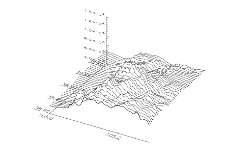
5. Use the AX keyword to rotate the plot 60 degrees along the x-axis and use the AZ keyword to rotate it –30 degrees along the z-axis:
SURFACE, elev, lon, lat, XStyle=1, CharSize=1.75, $
/Horizontal, Bottom=WoColorConvert(7), AZ=-30, AX=60
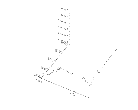
SURFACE, elev, lon, lat, XStyle=1, CharSize=1.75, $
/Horizontal, Bottom=WoColorConvert(7), AZ=-30, $
AX=60, /Lower_Only
SURFACE, elev, lon, lat, XStyle=1, CharSize=1.75, $
/Horizontal, Bottom=WoColorConvert(7), Skirt=5000
Display Data as a Shaded Surface
To view a 2D array as a light-source shaded surface, do the following:
1. First, enlarge the current window:
WINDOW, 0, XSize=800, YSize=800
2. Load one of the pre-defined PV-WAVE colortables by entering:
LOADCT, 5
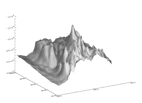
3. To view the light-source shaded surface, simply enter the command:
SHADE_SURF, elev, lon, lat
SURFACE, elev, lon, lat, XStyle=4, YStyle=4, ZStyle=4, $
Color=WoColorConvert(0), /Horizontal, /NoErase
note | The NoErase keyword allows the SURFACE plot to be drawn over the existing SHADE_SURF plot. The XStyle, YStyle, and ZStyle keywords are used to select different styles of axes. Here, SURFACE is told not to draw the x-, y-, and z-axes because they were already drawn by the SHADE_SURF command. |
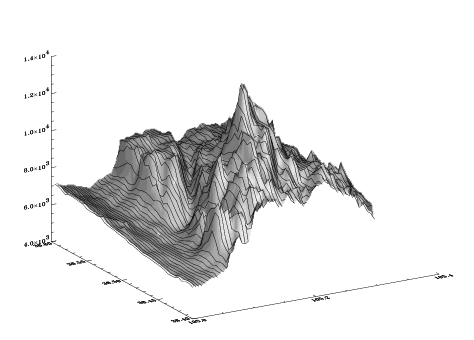
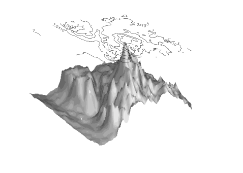
You can plot the contour lines on the shaded surface, but you will need to save the 3D transformation matrix using the Save keyword.
5. Draw the shaded surface without axes and save the transformation:
SHADE_SURF, elev, lon, lat, XStyle=4, YStyle=4, ZStyle=4, $
/Save
6. Now draw the contour lines on the current plot:
; Create a variable to specify the contour levels to display:
level = [5000, 6000, 7000, 8000, 9000, 10000, 11000, 12000]
CONTOUR, elev, lon, lat, XStyle=4, YStyle=4, ZStyle=4, $
/NoErase, Levels=level, /Follow, /T3D
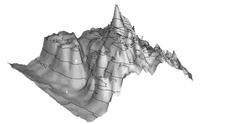
7. Now place colored contour lines above the shaded surface. When you loaded colortable 5, you overrode the TEK_COLOR palette, so you need to load it again:
TEK_COLOR
8. Draw the contour lines in colors. Place them above the shaded surface by specifying displacement along the z-axis (ZValue) of 1.0:
SHADE_SURF, elev, lon, lat, XStyle=4, YStyle=4, $
ZStyle=4, /Save
CONTOUR, elev, lon, lat, XStyle=4, YStyle=4, ZStyle=4, $
/NoErase, Levels=level, C_Colors=WoColorConvert(2), $
/Follow, /T3D, ZValue=1.0
Use Color to Represent Data
You can specify a different array for the shading colors.
1. Use TEK_COLOR again to load 32 distinct colors at the beginning of the current colortable:
TEK_COLOR
2. Find the BYTSCL values of the depth and allow the first 32 distinct values to be excluded:
shade = BYTSCL(depth, Top=222) + 32b
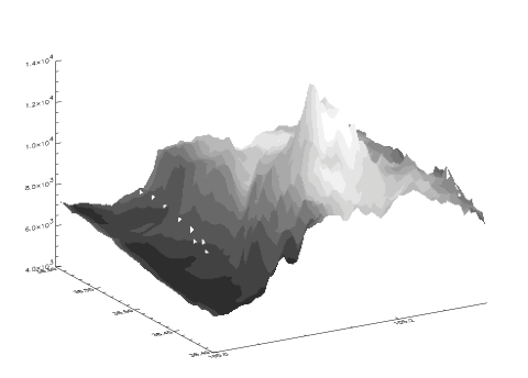
3. Shade the elevation data plot with snow depth values:
SHADE_SURF, elev, lon, lat, XStyle=1, Shades=shade, $
Color=WoColorConvert(1)
note | The BYTSCL function scales and converts an array to BYTE data type. The Shades keyword specifies the same dimensions as the shade parameter, which contains the shading color indices. |
The axes’ labels were drawn in white because this was specified by assigning the value of 1 (white in the TEK_COLOR palette) to the Color keyword.
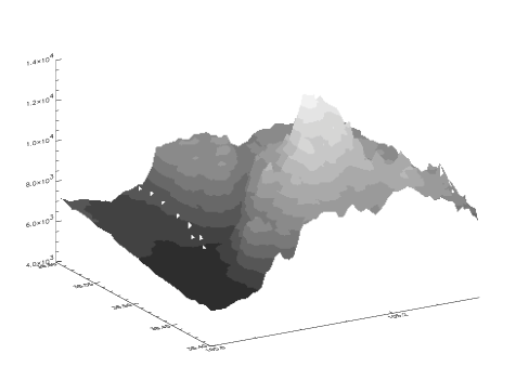
4. Create a shaded surface that has the shading information provided by the elevation of each point:
shade = BYTSCL(elev, Top=222) + 32b
SHADE_SURF, elev, lon, lat, XStyle=1, Shades=shade, $
Color=WoColorConvert(1)
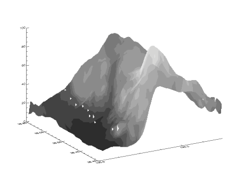
5. Shade the snow depth data plot with elevation:
SHADE_SURF, depth, lon, lat, XStyle=1, Shades=shade, $
Color=WoColorConvert(1)
More Information on 3D Plotting
The SURFACE, CONTOUR, and SHADE_SURF commands have many more keywords that can be used to create even more complex, customized plots. For more information see the PV‑WAVE User’s Guide.
Version 2017.1
Copyright © 2019, Rogue Wave Software, Inc. All Rights Reserved.