Frequency Domain Techniques
Filtering in the frequency domain is a flexible technique that is used for smoothing, sharpening, deblurring, and image restoration. The three basic steps in image filtering are:

Transforming the image into the frequency domain.
Multiplying the resulting complex image by a filter that usually has only real values.
Re-transforming this product back into the spatial domain, yielding the filtered image.
Assuming that A is the image to be filtered and filter is the variable containing the filter, this process is expressed by:
result = FFT(FFT(A, -1) * filter, 1)
The variable A may be of any data type except string; filter is a floating type filter and has the same dimensions as A; and result is the resulting image which is of complex type and has the same size as A. The second parameter of FFT specifies the direction of the transform: –1 for space to frequency; and +1 for frequency to space.
This process is equivalent to convolving the image with the spatial equivalent of the filter in the spatial domain, but is much quicker than simple convolution for kernels larger than approximately 9-by-9.
note | Try to avoid wrap-around artifacts when filtering and convolving in the frequency domain. In particular, images must be properly windowed and sampled before applying the Fourier Transform or false and misleading values will result. For one example of windowing, see the source code for the HANNING procedure in the Standard Library. |
Filtering Images
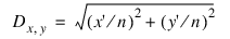
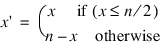
Many types of images can be improved by filtering. PV‑WAVE’s array-oriented operators and functions make it particularly easy to design and use filters. Many commonly used filters take advantage of what is called the frequency image. The frequency image, D, of an n-by-n array in which each pixel element contains the spatial frequency of the pixel in units of cycles per pixel is given by:
where:
The Standard Library function DIST evaluates the function above and returns a frequency image. For example, to obtain a frequency image to use with a filter for a 256-by-256 image, use the command:
D = DIST(256)
Some of the many filters which can be computed from the frequency image in one step are given below. The mathematical description of the filter is given first, followed by the PV‑WAVE code to implement it.
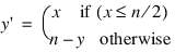
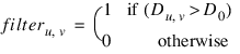
Ideal low pass filter, absolute cutoff at frequency
D0:
where filter = D LT D0.
Ideal high pass filter, absolute cutoff at
D0:
where filter = D GT D0.
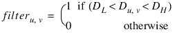
Ideal bandpass filter, absolute cutoff at
DL and
DH:
where filter = (D GT DL) AND (D LT DH).
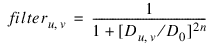
Butterworth low pass filter of order
n, cutoff at
D0: (The frequency response at the cutoff frequency is equal to 50% of the maximum.)
where filter = 1/(1+(D/D0) ^(2*N)).
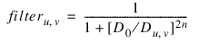
Butterworth high pass filter of order
n, cutoff at
D – 0:
where filter = 1/ (1 + (D0/D) ^ (2*N)).
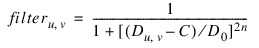
Butterworth bandpass filter, order
n, center frequency is C, width of
D0:
where filter = 1/ (1+((D-C)/D0) ^ (2*N)).
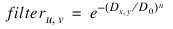
Exponential low pass filter of order
n:
where filter = EXP(-(D/D0) ^ N).
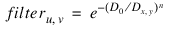
Exponential high pass filter of order
n:
where filter = EXP(- (D0/D) ^ N).
The filters described here must be applied in the frequency domain. To use these filters the image must be transformed to the frequency domain with the Fast Fourier Transform, multiplied by the filter, and then transformed back to the spatial domain.
The following command is used to apply a filter to the variable image:
filtered_image = FFT(FFT(image, -1) * filter, 1)
Displaying the Fourier Spectrum
PV‑WAVE makes it easy to calculate the Fourier spectrum of an image.
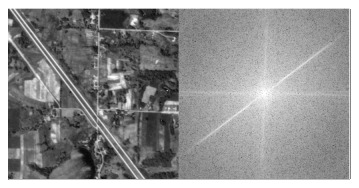
Aerial Image and its Fourier Spectrum shows an aerial photograph on the left and its logarithmically scaled Fourier spectrum on the right. Note that the diagonal, vertical, and horizontal lines in the Fourier spectrum correspond to the roads in the original image and are perpendicular to them.
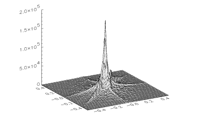
The Fourier spectrum is also displayed in
Surface Plot of Aerial Image as a surface plot.
It is customary to display the Fourier or power spectrum of images with the DC frequency component in the center of the image, as is done here. This is easily accomplished by using the SHIFT function to shift the origin of the 256-by-256 image to the center. The Fourier spectrum in the right side of
Figure 6-3: Aerial Image and its Fourier Spectrum on page 145 is produced with the statement:
TVSCL, SHIFT(ALOG( ABS( FFT(A, -1))),256, 256)
This statement performs the following operations:
The FFT function transforms the image into the frequency domain.
The ABS function calculates the magnitude of each complex-valued pixel.
The ALOG function returns the natural logarithm of each pixel.
The SHIFT function shifts the image so the point with a subscript of
(0, 0) is in the center.
The TVSCL procedure scales and displays the result.
Version 2017.1
Copyright © 2019, Rogue Wave Software, Inc. All Rights Reserved.