Geometric Transformations
Geometric transformations rearrange the elements of an image. Some examples of commonly used geometric transformations are: magnification, rotation, projection to different coordinate systems, and correction of distortions.
The definition of a geometric transformation may be written:
g(x, y) = f(u, v) = f[a(x, y), b(x, y)]
where f(u, v) is the input image, g(x, y) is the output image, and functions a and b specify the spatial transformation that relate the (x, y) coordinate system of the output image to the (u, v) coordinates of the input image.
Rotating and Transposing with the ROTATE Function
The simple and common operations of rotation by multiples of 90 degrees and/or transposition are performed most efficiently by the ROTATE function. The calling sequence for the ROTATE function is
ROTATE(image, rotation)
where image is the input array and rotation is an integer value specifying one of the eight possible combinations of axis interchange and reversal.
Example of ROTATE Function Usage
For example, a 90 degree counterclockwise rotation of an m-by-n image is expressed in the above notation by:
rotated_image = ROTATE(image, 1)
You can also use the ROT function to rotate an image. It uses POLY_2D (described in the next section) to rotate an image about a specified point with optional magnification or reduction. The rotation angle is not restricted to multiples of 90 degrees as in ROTATE, but ROT is slower. For more information on these functions, see the PV‑WAVE Reference.
Geometric Transformations with the POLY_2D Function
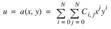
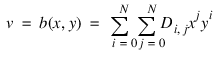
The POLY_2D function provides an efficient method of performing geometric transformations, assuming the functions a and b can be expressed as N-degree polynomials of x and y:
Either the nearest neighbor or bi-linear interpolation methods may be selected. The calling sequence and a brief description of the input parameters for the POLY_2D function is as follows.
output_image = POLY_2D(image, c, d[, interp[, dimx, dimy]])
Where:
 image
image—The input image.
c and
d—Arrays containing polynomial coefficients. Each array must contain (N + 1)
2 elements. For example, for a linear transformation
C and
D contain four elements, and may be a two-by-two array or a four-element vector.
Ci,j contains the coefficient used to determine
u, and is the weight of the term
xiyi. The POLYWARP procedure may be used to fit (
u,
v) as a function of (
x,
y). It returns the coefficient arrays
C and
D.
interp—If present and non-zero, selects bi-linear interpolation, otherwise the nearest neighbor method is used. For the linear case (i.e.
N = 1) bi-linear interpolation requires approximately twice as much time as does the nearest neighbor method.
dimx and
dimy—Specify the dimensions of the result. If omitted, the result will have the same dimensions as the original image.
In addition, the output keyword parameter Missing may be included to specify the output value of pixels whose u, v coordinates are outside the input image. If this keyword parameter is not present, missing values are extrapolated from the edges of the input image. For more detailed information on the POLY_2D function, refer to the function description in the PV‑WAVE Reference.
Efficiency and Accuracy of Interpolation
POLY_2D is relatively efficient; however, some of this efficiency is gained at the expense of accuracy. Each output pixel is mapped to the input image and the nearest pixel is used for the result. This method is called the nearest neighbor method. With high magnifications of regular structure, objectionable sawtooth edges result. bi-linear interpolation avoids this effect by determining the value of each output pixel by interpolating from the four neighbors of actual location in the input image at the expense of additional computations.
Correcting Linear Distortion with Control Points
The following example uses POLY_2D to correct a linear distortion using control points. A calibration image containing n known points is acquired by a system with linear distortion. Given the original position of each point in the calibration image, (x, y) and its measured coordinates in the acquired image, (u, v), it is possible to obtain the polynomial coefficients required to transform the acquired image back to the original.
The value of
n must be at least four to determine the coefficients of a first degree transformation, as there are (
n + 1)
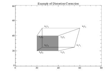
2 coefficients in each array, each of which is an unknown to be solved. In this example, four points are measured which describe the pixel coordinates of the corners of a box in the undistorted calibration image: (20, 20), (40, 20), (40, 40), (20, 40). The measured coordinates of the corners of the box, which is distorted into the shape of a trapezoid in the acquired image, are assumed to be: (25, 25), (55, 25), (60, 50), (25, 50). See
Figure 6-5: Geometric Distortion on page 149.
The equations relating the (u, v) coordinates to (x, y) are:
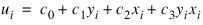
, i
= 0, 1, 2, 3 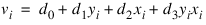
, i
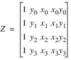
= 0, 1, 2, 3 We can write the four equations for ui as:
U = ZC
where C = [c0, c1, c2, c3], and:
Solving for C and D:
C = Z–1U D = Z–1V
The statements implementing this algorithm are:
; Define undistorted x coordinates of box.
x = [20, 40, 40, 20]
; ... and y.
y = [20, 20, 40, 40]
; Measured coordinates...
u = [25, 55, 60, 25]
v = [25, 25, 50, 50]
; Define the Z matrix.
z = FLTARR(4,4)
; Fill it, one row at a time.
FOR j=0,1 DO for k=0,1 DO z(0,j+2*k) = x^k * y^j
; Create a 100-by-100 image.
image = BYTARR(100, 100)
; Simulate acquired image by filling pixels inside (u, v) box
; with the value 128.
image(POLYFILLV(u, v, 100, 100)) = 128
; Solve the equations, using the INVERT function, and
; apply the geometric transformation, yielding image q, saving
; coefficients in c and d.
q = POLY_2D(image, (c = INVERT(z) # u), (d = INVERT(z) # v), 1)
The computed values of c and d are [0.0, –0.25, 1.25, 0.0125], and [0.0, 1.25, 0.0, 0.0 ].
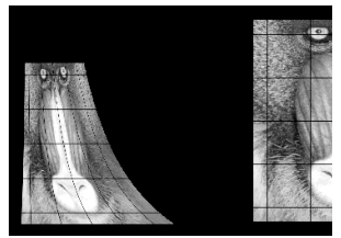
Correcting a Geometric Transformation illustrates the application of this geometric transformation to an image. The left side of this figure contains the trapezoid defined by the distorted coordinates of the “acquired” image. The right side is the result of the transformation, as the trapezoid is warped back to the original rectangular shape.
The POLYWARP procedure may be used to obtain the polynomial coefficients in a more general manner. It is not restricted to first- order polynomials, and it computes a least squares fit if there are more than (n + 1)2 control points. For more information on the POLYWARP procedure, see its description in the PV‑WAVE Reference.
Version 2017.1
Copyright © 2019, Rogue Wave Software, Inc. All Rights Reserved.