Creating Plots with Date/Time Data
The plotting procedures, PLOT and OPLOT, in conjunction with keywords can be used to plot multiple date/time labels and tick levels on the x-axis. The keywords for the PLOT procedure for date/time include:
 XType
XType Start_Level Month_Abbr Box DT_Range Max_Levels Compress The keywords for OPLOT are XType and Compress. You can find a complete description of all these keywords in Chapter 21: Graphics and Plotting Keywords in the PV‑WAVE Reference.
The following examples show eight different types of plots with date/time axes.
Example 1: Plotting Seconds
This example illustrates how to generate a date/time plot for a data file named datafile.dat that does not contain explicit date and time information, that is, no time stamp information. The file contains data for every second of the day for April 1, 1992. The one-column file looks like:
00.355187
91.9201
00.22395
63.9256
97.4526
.
.
.
The following code generates a plot that shows the first seven seconds of data, as shown in
Figure 8-2: Date/Time Plot for April 1, 1992 on page 228. The date/time axis is shown with the maximum of six labels.
; Generates an initial date/time variable to use with the
; DTGEN function.
fday = VAR_TO_DT(1992, 4, 1, 1, 1, 1)
; Creates a variable for generating seven seconds of data.
num = 7
; Generates date/time variable with date/time structures for the
; first seven seconds of April.
x = DTGEN(fday, num, /Second)
; Reads the data from the file datafile.dat and assigns it to the
; variable y. The values for all seconds, 86400, are actually
; read into y. However, only the first seven seconds are plotted
; for this example.
status = DC_READ_FREE('datafile.dat', y, /Col); Plots the first seven seconds of data.
PLOT, x, y, Psym = -4
Example 2: Plotting Minutes
The second example uses the same data file as Example 1 (
datafile.dat). The example shows how you can plot a graph for the data at each minute rather than each second. The
Box keyword draws boxes around the tick marks and labels of the date/time axis. The results are shown
Date/Time Plot for First Twenty Minutes.
; Generates an initial date/time variable to use with the
; DTGEN function.
fday = VAR_TO_DT(1992, 4, 1, 1, 1, 1)
; Creates a variable to use with the DTGEN function for generating
; an array of date/time structures.
num = 20
; Generates a date/time variable with date/time structures for
; 20 minutes in April.
x = DTGEN(fday, num, /Minute)
; Reads the data from the file datafile.dat into the variable y.
status = DC_READ_FREE('datafile.dat', y, /Col); Plots the first 20 minutes of data with boxes around the
; date/time axis.
PLOT, x, y, Psym=-4, /Box
If no boxes are drawn for the date/time axis, labels are centered with respect to the tick marks for seconds, minutes, hours, and days. Weeks, months, quarters, and years are always left-justified. See Example 1. With boxes, the labels are left-justified in relation to the tick marks.
Example 3: Plotting Hourly Data
The third example uses the same data file as Examples 1 and 2. This example plots data for every hour of the day April 1, as shown in
Date/Time Plot at each Hour.
; Create an initial date/time variable to use with the DTGEN
; function.
fday = VAR_TO_DT(1992, 4, 1, 1, 1, 1)
; Create a variable used with the DTGEN function to create an
; array of date/time structures.
num = 24
; Create 24 date/time structures for the hours of the day.
x = DTGEN(fday, num, /Hour)
; Read the data into the variable y.
status = DC_READ_FREE('datafile.dat', y, /Col)Plot, x, y, Psym = -4, /Box
Example 4: Plotting Daily Sales Data
Examples 4 through 8 plot date/time data for a file named sales1.dat that contains date/time stamps for product sales. The file has ten columns. Each data set column has an accompanying date stamp column:
Product Sales
Daily Weekly Monthly Quarterly Yearly
00 1/01/1991 159 1/06/91 1088 1/31/91 3000 910101 5280 85941
91 1/02/1991 152 1/13/91 1085 2/28/91 1942 910401 6581 86307
05 1/03/1991 202 1/20/91 0827 3/31/91 . .
. . . 2345 911001 7621 87037
. . 1147 12/31/31
. 150 12/31/91
57 12/31/1991
note | This data file is an example file only. It is used to generate plots for various levels of date/time data. |
Example 4 plots the daily sales for the month of January. Weekend days are compressed with the keyword
Compress. The
DT_Range keyword is used to plot a portion of the date/time data read in from the file. The results are shown in
Figure 8-5: Date/Time Plot for Daily Product Sales on page 232.
; Create date/time structures to hold date/time data for the days
; in January and February.
dates = REPLICATE({!DT}, 60); This procedure defines the weekend days.
CREATE_WEEKENDS, ['sun', 'sat']
; Reads the data from Column 1 into the variable amount. Reads
; the data from Column 2 into the variable dates. The date/times
; from Column 2 are converted to date/time data. The NSkip keyword
; skips over the first two header lines in the file.
status = DC_READ_FREE('sales1.dat', amount, dates, /Col, $
Dt_Template = [1], Delim = [" "], NSkip = 2, $
Get_Columns = [1, 2])
; Creates variables to be used with DT_Range. These variables
; establish a range for plotting each day of month in January.
sdate = VAR_TO_DT(1991, 1, 1)
edate = VAR_TO_DT(1991, 1, 30)
; Plots the date/time data on the x-axis and the daily sales for
; the month of January on the y-axis. Weekends are compressed.
; Setting the Start_Level keyword to 3 forces the plot to use
; days as the first axis level. The DT_Range keyword defines the
; range of date/time data that will be plotted. In this example
; only the days of January are plotted.
PLOT, dates, amount, /Compress, Start_Level = 3, $
DT_Range = [sdate.julian, edate.julian]
Example 5: Plotting Sales Per Week
Example 5 plots the weekly sales from January 1 to May 6. The data and date/time are read in from Columns 3 and 4 of
sales1.dat. The results are shown in
Figure 8-6: Date/Time Plot from January 7 to May 6 on page 233.
; Create date/time structure to read date/time data into.
dates = REPLICATE({!DT}, 18); Read sales data into the amount variable. Read and convert
; date/time data into the dates variable.
status = DC_READ_FREE('sales1.dat', amount, dates, /Col, $
Dt_Template = [1], Delim = [" "], Get_Columns = [3,4], $
NSkip = 2)
; The keyword Start_Level selects weeks for plotting.
PLOT, dates, amount, Start_Level =4, PSym = -4
note | By default, week boundaries are plotted as Mondays. To label a different day of the week, use the Week_Boundary keyword. To specify an exact axis range, use the Dt_Range keyword. Looking at the above example, to have the tick labeling occur on the day of the week of the first data point, and to plot only the first 12 weeks of data use the following: PLOT,dates,amount,Start_level=4, Psym=-4, $
Dt_Range=[dates(0).Julian,dates(12).Julian], $
Week_boundary=DAY_OF_WEEK(dates(0)) |
Example 6: Plotting Monthly Sales
Example 6 plots the total sales for each month, as shown in
Figure 8-7: Monthly Sales Plot on page 234. This data is contained in Columns 5 and 6 of
sales1.dat. The keyword
Month_Abbr automatically abbreviates some month names to three characters depending on the available space on the axis. In this example, no labels would be shown for the months of February or September without this keyword.
; Creates date/time structures for the months of the year.
dates = REPLICATE({!DT}, 12); Reads monthly sales data into the amount variable. Reads
; date/time data into the variable dates as date/time data.
status = DC_READ_FREE('sales1.dat', amount, dates, /Col, $
Dt_Template = [1], Delim = [' '], NSkip = 2, $
Get_Columns = [5,6])
; Plots data with several months abbreviated to fit labels for
; all 12 months on the date/time axis.
PLOT, dates, amount, /Month_Abbr
Example 7: Plotting Quarterly Sales
This example plots the data from Columns 7 and 8 of the sample file sales1.dat. The date information is not in any format that can be used with the DT_Template keyword. Therefore, the dates are first read and then converted using the VAR_TO_DT function.
The
Start_Level keyword insures that the quarterly sales are printed out on the first level. The
Max_Levels keyword defines one level of axis labels. An OPLOT is also shown for the projected sales for each quarter of the year (the individual diamonds in
Quarterly Sales Plot). The OPLOT does not generate any tick marks or labels; you can only plot a second set of data on the original date/time axis.
; Creates variables to hold the date information for the four
; quarters of the year.
year = intarr(4) & month = intarr(4)
day = intarr(4)
; Reads the sales data into the amount variable. Reads the
; date information into the variables, year, month, and day.
status = DC_READ_FIXED('sales1.dat', amount, year, month, day, $
/Col, NSkip = 2, FORMAT = ('39X, I4, 1X, 3I2)')
; Converts the date information to a date/time variable.
dates = VAR_TO_DT(year, month, day)
; Plots the data with only one level of axis labeling.
; Without the Max_Levels keyword assignment, the labels
; for years would also be printed out.
PLOT, dates, amount, Start_Level = 6, /Max_Levels
; These are the projected sales for each quarter of 1991.
amount1 = [3507, 2310, 2917, 1807]
; Plots projected sales of each quarter as individual diamonds.
OPLOT, dates, amount1, PSym = 4
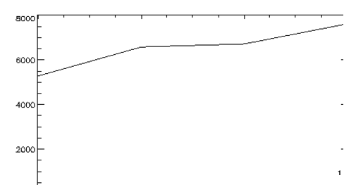
Example 8: Plotting Yearly Sales
Example 8 plots the data from Columns 9 and 10 of
sales1.dat. The Julian dates are supplied in Column 10. Column 9 contains the sales for each of the last four years, as shown in
Yearly Sales Plot over Four Years.
; Defines the d variable as a long array containing 4 elements.
; This variable contains the Julian dates read in from Column 10.
d = lonarr(4)
; Reads the sales data into the amount variable. Reads the
; date information into variable d.
status = DC_READ_FREE('sales1.dat', amount, d, /Col, $
Delim = [" "], NSkip = 2, Get_Columns = [9, 10])
; Converts date information in variable d to date/time variable.
dates = JUL_TO_DT(d)
; Plots yearly sales. The Start_Level keyword ensures that the
; years are labeled on the first level of the x-axis. If this
; keyword were omitted, quarters would be the first level of
; labeling.
PLOT, dates, amount, Start_Level = 7
Example 9: Plotting Yearly Sales with the XType Keyword
PV‑WAVE provides another method for plotting date/time data if your file contains Julian days as in Example 8. You can set the XType plot keyword to a value of 2 to generate a date/time axis. Since the Julian days are provided in Column 10 for the yearly sales data in Column 9, you can plot these two columns as follows:
; Defines dates variable as a long array containing 4 elements.
dates = LONARR(4)
; Reads the sales data into the amount variable.
; Reads the date information into the dates variable.
status = DC_READ_FREE('sales1.dat', amount, dates, /Col, $
Delim = [" "],   Get_Columns = [9, 10], NSkip = 2)
; Plots data as shown in
;
    Figure 8-9: Yearly Sales Plot over Four Years on page 236.
PLOT, dates, amount, XType=2, Start_Level=7
See Chapter 21: Graphics and Plotting Keywords in the PV‑WAVE Reference for more information about the XType keyword. Also see the description of the DT_COMPRESS function in the PV‑WAVE Reference.
Version 2017.1
Copyright © 2019, Rogue Wave Software, Inc. All Rights Reserved.