Mapping
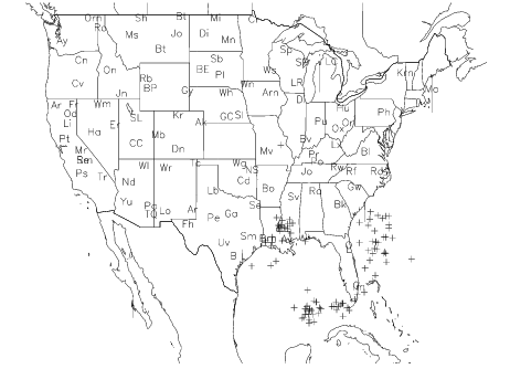
The PV‑WAVE mapping procedures let you create a variety of mapping applications. Scientific data, economic data, aerial photography data, and other kinds of data can be plotted with maps generated by PV‑WAVE, as shown in
Lightning Strikes in the US.
This section discusses how to use the PV‑WAVE mapping procedures.
Mapping Procedures
Typical uses for the PV‑WAVE mapping procedures include:

Scientific applications where wide-area data is plotted with coastline and political boundaries.
Business applications where geographic data is displayed and highlighted to reflect a measured quantity.
Military, environmental, and remote sensing applications where satellite imagery and digitized aerial photography are integrated with maps.
The mapping procedures, map datasets, and demonstration files are located in the PV‑WAVE mapping directory:
(UNIX) <RW_DIR>/mapping-2_0
(WIN) <RW_DIR>\mapping-2_0
Where <RW_DIR> is the main PV-WAVE installation directory.
The PV‑WAVE mapping procedures can be adapted easily to work with your own projections and map datasets. The mapping procedures include:
MAP—Plots map data with a specified projection.
MAP_CONTOUR—Plots contours on a map.
MAP_LAND—For each map pixel, identify longitude, latitude, and cover type.
MAP_PLOTS—Plots vectors or points on the current map projection.
MAP_POLYFILL—Fills specified regions of a map.
MAP_REVERSE—Converts X-Y coordinate data to longitude and latitude coordinates.
MAP_VELOVECT—Plots a two-dimensional vector field on a map.
MAP_XYOUTS—Adds text to a map.
USGS_NAMES—Queries a database of longitude/latitude coordinates for states, counties, cities, and towns in the United States.
Using Map Projections and Datasets
This section highlights some of the concepts that are central to using the PV‑WAVE mapping routines.
For more information on mapping projections and in-depth discussions of algorithms and uses of the projections PV‑WAVE generates, refer to the following publications:
Map Projections Used by the U.S. Geological Survey, Geological Survey Bulletin 1532, John P. Snyder, Second Edition, 1983.
An Album of Map Projections, U.S. Geological Survey Professional Papers 1453, John P. Snyder and Philip M. Voxland, 1989.
Both are available from:
USGS Information Services
Box 25286
Denver, CO USA 80225
Phone: (303) 1-888-ASK-USGS
FAX: (303) 202-4693
www.usgs.gov What Are Map Projections?
A central problem facing cartographers for centuries was how to represent the features of a spherical globe on a flat map. The methods devised for “flattening” the globe onto a map are called map projections. PV‑WAVE can generate 17 different types of projections. It is also possible for you to design your own algorithms and use them in PV‑WAVE.
A map projection transforms spherical coordinates into two-dimensional X-Y coordinates. The spherical coordinates of the globe are defined by lines of longitude and latitude.
Longitude is the angle in degrees east or west of the prime meridian passing through Greenwich, England, and latitude is the angle in degrees north or south of the Equator.
For more information on the types of map projections included in PV-WAVE, please refer to the PV‑WAVE User’s Guide.
What Are Map Datasets?
In PV‑WAVE a map dataset is a set of polylines (a series of connected points) or polygons (points which describe a filled area). These polylines or polygons can have a number of classification attributes associated with them which aid in selecting features to be plotted. These attributes allow the desired polylines or polygons for a map to be selected based on the area being mapped and the features you want to plot.
For more information on the map datasets included in PV-WAVE, please refer to PV‑WAVE User’s Guide.
Reading Other Map Datasets Into PV-WAVE
The World Databank II and USGS Digital Line Graph datasets are provided with PV‑WAVE, as are procedures used to read them. To read another dataset other than World Databank II and USGS Digital Line Graph Dataset, you must write a procedure tailored to read that dataset.
Specifying a Map Projection
The Projection keyword for the MAP procedure lets you specify a projection for the map that is drawn. PV‑WAVE provides several built-in projections, but you can also add your own projection algorithm.
To specify a projection, set the
Projection keyword to the corresponding map projection index number. The map projections and their index numbers are shown in
Table 8-1: Map Projections in PV‑WAVE on page 143.
Version 2017.1
Copyright © 2019, Rogue Wave Software, Inc. All Rights Reserved.